TensorFlow.js Part 1 - Develop Model in Python

Update 23 October 2022: The model should be called an autoencoder, see discussion.

This post is part one of a three-part series in which we are going to explore how TensorFlow models can be integrated in website front-ends written in JavaScript with TensorFlow.js. This is useful if you want to run a small model, but don’t want to send client data to a server out of privacy concerns. TensorFlow.js can also be used in JavaScript on a backend which runs Node.js.

In this first part, we are going to develop and train a model with TensorFlow in Python. In part two we then export this model so that it can be used in TensorFlow.js. The last part explores how a converted model can be used in JavaScript. We develop a simple website with React.js which allows us to upload an image and run the model on it.

To follow along, you can download code here. If you want to dive into the Javascript part directly, you can also skip this part and use a model from the models folder.

Additionally, the content of this post is also available as a video:

Develop Model and Loss Function

We are going to build a simple fully convolutional network that will be trained with a pixel loss to reconstruct an input image. Such a model is used for example for real-time style transfer or image upscaling (super-resolution).

# Model.
def get_model():
    inputs = keras.Input(shape=(256,256,3), name="InputLayer")   
    x = layers.Conv2D(filters=32, kernel_size=(9,9), strides=(1,1), activation="relu", padding='same', name="Conv1")(inputs)
    x = layers.Conv2D(filters=64, kernel_size=(3,3), strides=(2,2), activation="relu", padding='same', name="Conv2")(x)
    x = layers.Conv2DTranspose(filters=32, kernel_size=(3,3), strides=(2,2), activation="relu", padding='same', name="Deconv1")(x)
    x = layers.Conv2DTranspose(filters=3, kernel_size=(9,9), strides=(1,1), padding='same', name="Deconv2")(x) 
    outputs = activations.tanh(x)   
    return keras.Model(inputs=inputs, outputs=outputs, name="fcn_model")

model = get_model()

Next, we define a pixel loss which takes the squared distance between two images based on their pixel values.

# Pixel loss.
def compute_pixel_loss(generated_image, original_image):
    return tf.reduce_sum(tf.square(original_image - generated_image))

Data

To train the model, we use a few images which can be found in the data folder. For this demo, you can use as many images as you like since we are not interested in making a good model, but rather want to explore how to use models in TensorFlow.js. I used four images from the COCO dataset. The model is going to overfit on those, and that is totally fine for this tutorial.

To load data from the folder we define an image_dataset.

# Make TensorFlow dataset.
image_size = (256,256)
batch_size = 1

image_path = "./data/"

train = keras.preprocessing.image_dataset_from_directory(
    image_path,
    labels=None,
    image_size=image_size,
    batch_size=batch_size
)

Training Loop

To train the model we need one more piece: a training loop which takes images, runs a forward pass, evaluates the output with the loss function, and updates the weights with the gradients.

# Compute loss and gradients for training loop.
@tf.function
def compute_loss_and_grads(original_image):
    """
    Takes in content and style images as tf.tensors with batch dimension
    and scaled to range [0,1].
    """
    
    with tf.GradientTape() as tape:
        # Forward pass
        generated_image = model(original_image, training=True)
        
        # Convert to range [0,1]
        generated_image = ((generated_image * 0.5) + 0.5)

        # Get loss
        loss = compute_pixel_loss(generated_image, original_image)

    # Get gradients and upate weights
    grads = tape.gradient(loss, model.trainable_weights)
    optimizer.apply_gradients(zip(grads, model.trainable_weights))
    return loss

The function decorator @tf.function compiles the function into a static graph which means for us that it runs faster.

With the function above, we can finally define the training loop.

# Train model.
num_epochs = 200
optimizer = keras.optimizers.Adam(learning_rate=0.001)

model = get_model()

for epoch in range(num_epochs):
    print("Running epoch %d / %d" %(epoch+1, num_epochs))
    for step, img in enumerate(train):
        
        # Scale image to range [0,1]
        img = img / 255.0
        loss = compute_loss_and_grads(img)

model.save("./models/fullyConvolutionalModel")

After running the loop, the model is saved to the models folder. With the command model.save() we save the model in the SavedModel format. An alternative is the Keras HDF5 format which requires different commands later.

Check model

Finally, we can check if the model we just trained can reconstruct the images.

def generate_image(image_name):
    """
    Runs inference with selected image and displays result.
    """
    base_path = "./data/"  
    image = keras.preprocessing.image.load_img(base_path + image_name + ".jpg")  
    image = keras.preprocessing.image.img_to_array(image)
    
    # Preprocess image. Final shape is (batch, height, width, colour).
    image = tf.image.resize(image, [256, 256])
    image = image / 255.0
    image = np.array([image])

    # Convert to TensorFlow tensor.
    image = tf.convert_to_tensor(image)   
    generated_image = model(image, training=False)
    generated_image = generated_image.numpy()
    generated_image = ((generated_image * 0.5) + 0.5) 
    generated_image = generated_image * 255

    # Remove batch dimension and show.
    generated_image = generated_image.reshape((256,256,3))
    img = ImagePIL.fromarray(np.uint8(generated_image)).convert('RGB')
    display(img)
generate_image("000000487217")

Figure 1: Image reconstructed with the test model.

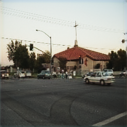
Figure 1 shows the result from the image which is in the data folder. As you can see it looks pretty good! This is no surprise since the model memorized this image due to lack of data, but it will do for this demo.