Evaluation Metrics
Before getting into how object recognition models work, it would first be useful to know how to evaluate the performance of these models so that they may be compared. To explain this, we first give a recap on evaluating a binary classification system. Then we show how the case of binary classification can be expanded to multiclass object detection. Finally, we introduce a popular metric used to evaluate object detection models: mean average precision (mAP).
Metrics for binary classification
The simplest and most obvious way to evaluate a binary classifier model is to measure its accuracy which is the simple ratio of the number of correct predictions to the total number of predictions:
\begin{equation} \tag{1.1} Accuracy = \frac{Y_{correct}}{Y_{total}} \end{equation}
Accuracy works very well for balanced or near balanced datasets where the number of positives and negatives are approximately the same. However, real world data is often skewed to have a lot more negatives than positives which leads to a problem using accuracy to evaluate a model. Suppose you are a weather forecaster predicting whether it is going to rain tomorrow. Your predictions are \(98\%\) accurate. Normally, this would be very impressive. But suppose you are predicting the weather in a desert where the average chance of rain is \(2\%\) (that is there are \(2\%\) positives in the dataset). You could achieve \(98\%\) accuracy by just always predicting that will not rain. Predicting rain would probably hurt your accuracy because by chance it is far likelier for it to be sunny, so you’d have to be fairly confident that it would rain the next day to improve your accuracy.
This example shows that when dealing with unbalanced data, metrics which distinguish between the types of error the model makes on the positive class are more helpful. This is where precision and recall come into play. Precision quantifies the number of correct predictions of the class we are interested in (positive class):
\begin{equation} \tag{1.2} Precision = \frac{TP}{TP + FP} \end{equation}
Here TP are true positives, meaning samples of the positive class which are predicted as such. FP is a false positive, which is a negative sample falsely predicted as positive.
On the other hand, recall is the number of positives the model finds out of all existing positives in the dataset (that is all TPs and the falsely as negative classified positives, FN):
\begin{equation} \tag{1.3} Recall = \frac{TP}{TP + FN} \end{equation}
To illustrate how these metrics work, let’s look at some extreme examples. Assume we have a model which correctly predicts one positive on a dataset with a moderate number of positives. This model is very confident in its one positive prediction and easily makes this prediction correctly. Here the precision is \(1\) and the recall is close to \(0\) due to the high number of missed positives (FN), see equation (1.3). On the opposite side of the spectrum, the model can assign every prediction a positive label. This means this model would have a perfect recall of $1$ while a fairly low precision because of all the false positive predictions. Ideally, a perfect model which doesn’t make any mistakes achieves both a precision and recall of \(1\).
In reality there is a trade-off between the two metrics. So given a trained model, how can we influence precision and recall? Suppose you have a machine learning classifier with an output range \([0,1]\) which represents a confidence score, like logistic regression. Typically, if an output is greater than a threshold of \(0.5\) we consider it a positive prediction, otherwise a negative prediction. However, this threshold is arbitrary and we can choose it to be something else. By increasing the threshold for example we can make the model output more confident predictions in the positive class. This leads to an increased precision at the cost of on average lowered recall.
As you can see both of these metrics are important when evaluating models. Since it is difficult to compare models using two metrics, they can be combined into the F1 score:
\begin{equation} \tag{1.4} F1 Score = 2 \cdot \frac{Precision*Recall}{Precision+Recall} \end{equation}
Error types in object detection
The metrics mentioned so far are used to quantify errors made on the positive class in binary classification problems and suited for dealing with imbalanced datasets. For object detection in particular, the terms mean Average Precision (mAP) and Intersection over Union (IoU) are often used in relation to evaluating models.
In object detection tasks, objects are identified by placing bounding boxes around them and assigning a label to each box. The label assignment can be framed as multiple binary classification problems of the respective ground truth class and background class as follows. For each object class we can construct a binary classification problem between the object class and background. Thus, when we have \(80\) object classes for example we would have \(80\) binary classification problems to assign the labels. Each of those are highly skewed towards the background class due to the way object detectors work (think of it as sliding a small window over the image and making a prediction for each possible position. Most predictions will contain background while few contain objects. More on this later.).
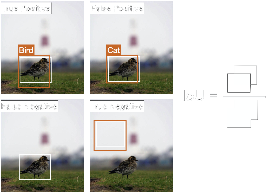
Figure 3 shows the four different error types for the example class “bird”. A true positive is when the predicted bounding box overlaps sufficiently well with the ground truth box, and both are associated with the same class. If the class differs, this is a false positive. If no box is predicted where a ground truth box is located, then it is a false negative. And finally, if a box correctly predicts no object (ground truth is background) it is a true negative. In object detection, however, true negatives are often ignored since we are interested in the location of objects, not the background. If a model outputs, for example, \(3\) boxes with the correct class label, one of them is deemed a true positive and the other two are considered false positives since the model failed to remove the duplicate predictions.
To measure if and how well a predicted bounding box overlaps with a ground truth box, the overlap is quantified using Intersection over Union. Given two boxes, IoU is their overlap divided by the total area of both boxes, see right side of figure 3. Typically, an \(IoU ≥ 0.5\) is considered correctly located. This low threshold accounts for some uncertainty in the annotating the bounding box [5].
Using these error cases, the precision and recall for each possible object class can then be calculated for a given confidence threshold and summarized in the precision recall curve, which we look at next.
Precision recall curve
Before we get to mean Average Precision we need one more piece; the precision recall curve. Above we mentioned the trade-off between precision and recall. In the absence of the cost of a misclassification it is difficult to find the right balance between precision and recall. That is why in order to evaluate a model we vary the confidence threshold and then plot the corresponding precision over the recall, see orange line in figure 4. Here, the optimal point is in the upper right corner, which is where the model makes no mistakes.
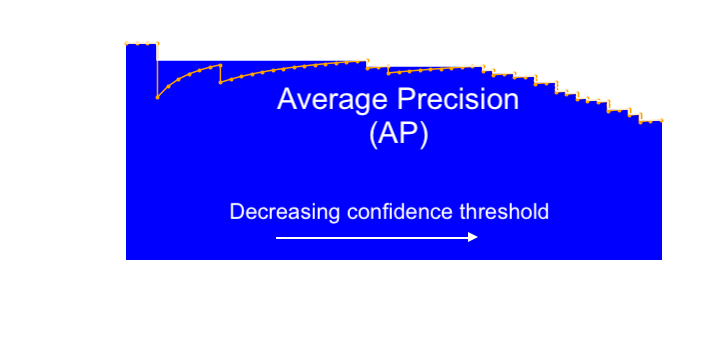
Let’s see what is going on here. When the confidence threshold is high, only a few positives are predicted, but the model is very confident about them. Thus, the recall is low and precision is high. Then you lower the threshold over and over again and observe. Starting from the top left of the curve, if the next sample when lowering the threshold turns a false negative to a true positive, this increases recall of the model, moving the curve rightwards. However, if lowering the threshold turns the next sample of a true negative into a false positive, the precision gets hit while the recall doesn’t change at all, moving the curve straight downwards. The next true positives will increase both recall and precision, causing the curve to move rightwards and creep upwards. This is why the curve has this sawtooth pattern with sudden drops and gradual increases moving rightwards. Sometimes this curve is smoothed out a bit by taking the highest precision for the current or greater recall (see white line in figure 4).
Precision and recall can then be united under a single metric: the area under the curve called Average Precision (AP). That means to achieve a high score, a detector must perform well on all examples and not only a subset. For example, a detector for vehicles must identify vehicles correctly from all view angles and scales which are present in the dataset, thus achieving high precision for all levels of recall. It is not sufficient to learn side views with very high confidence at the cost of lower confidence for far-field views from the rear. As a consequence, detectors are encouraged to generalize well to different scenarios.
To compare multiclass object detectors, the AP for each class is calculated and then averaged across the classes. This average over each class AP is known as the mean Average Precision (mAP): the score typically reported in object detection competitions.
Competition specific metrics
So far we have learned how models can be compared using mAP when acceptable levels of precision and recall for each class are unknown. We now look at how mAP is used and adapted to rank object detectors in the two influential benchmarks PASCAL and COCO.
PASCAL Object Detection
In the detection tasks of the PASCAL competition, the AP was calculated similar to what is explained above. A predicted bounding box is considered correctly located if the IoU is at least \(0.5\) and the associated label is correct [10]. For each class, the precision recall curve is then calculated by using the reported confidence levels for each prediction. However, here an interpolated AP is used which is calculated as follows.
First the recall levels are split into \(11\) equally spaced intervals. For each of these intervals, the precision \(p_{inter(r)}\) is taken to get the precision for each recall level:
\begin{equation} \tag{1.3} p(r) = \frac{1}{11} \sum_{r \in \{0,0.1,…,1\}} p_{inter}(r) \end{equation}
Here \(p_{inter}\) is the maximum precision in each recall interval:
\begin{equation} \tag{1.4} p_{inter}(r) = \max_{\widetilde{r}:\widetilde{r} ≥ r} p(\widetilde{r}) \end{equation}
Taking this interpolated precision has a smoothing effect similar to the white line in figure 4. This helps reduce the impact of small variations in the ranking of examples. The downside of this interpolation is that it makes it difficult to distinguish between results at low AP. That is why the interpolation was removed in 2010 and AP was reported from the unmodified curve [10].
| Class | CVC CLS | Missouri | NEC | OLB R5 | SYSU Dynamic | Oxford | UVA Hybrid | UVA Merged |
|---|---|---|---|---|---|---|---|---|
| Aeroplane | 45.4 | 51.4 | 65.0 | 47.5 | 50.1 | 59.6 | 61.8 | 47.2 |
| Bicycle | 49.8 | 53.6 | 46.8 | 51.6 | 47.0 | 54.5 | 52.0 | 50.2 |
| Bird | 15.7 | 18.3 | 25.0 | 14.2 | 07.9 | 21.9 | 24.6 | 18.3 |
| Boat | 16.0 | 15.6 | 24.6 | 12.6 | 03.8 | 21.6 | 24.8 | 21.4 |
| Bottle | 26.3 | 31.6 | 16.0 | 27.3 | 24.8 | 32.1 | 20.2 | 25.2 |
| Bus | 54.6 | 56.5 | 51.0 | 51.8 | 47.2 | 52.5 | 57.1 | 53.3 |
| Car | 44.8 | 47.1 | 44.9 | 44.2 | 42.8 | 49.3 | 44.5 | 46.3 |
| Cat | 35.1 | 38.6 | 51.5 | 25.3 | 31.1 | 40.8 | 53.6 | 46.3 |
| Chair | 16.8 | 19.5 | 13.0 | 17.8 | 17.5 | 19.1 | 17.4 | 17.5 |
| Cow | 31.3 | 31.9 | 26.6 | 30.2 | 24.2 | 35.1 | 33.0 | 27.8 |
| Diningtable | 23.6 | 22.1 | 31.0 | 18.1 | 10.0 | 28.9 | 38.2 | 30.3 |
| Dog | 26.0 | 25.0 | 40.2 | 16.9 | 21.3 | 37.2 | 42.8 | 35.0 |
| Horse | 45.6 | 50.3 | 39.7 | 46.9 | 43.5 | 50.9 | 48.8 | 41.6 |
| Motorbike | 49.6 | 51.9 | 51.5 | 50.9 | 46.4 | 49.9 | 59.4 | 52.1 |
| Person | 42.2 | 44.9 | 32.8 | 43.0 | 37.5 | 46.1 | 35.7 | 43.2 |
| Pottedplant | 14.5 | 11.9 | 12.6 | 09.5 | 07.9 | 15.6 | 22.8 | 18.0 |
| Sheep | 30.5 | 37.7 | 35.7 | 31.2 | 26.4 | 39.3 | 40.3 | 35.2 |
| Sofa | 28.5 | 30.6 | 33.5 | 23.6 | 21.5 | 35.6 | 39.5 | 31.1 |
| Train | 45.7 | 50.8 | 48.0 | 44.3 | 43.1 | 48.9 | 51.1 | 45.4 |
| Tvmonitor | 40.0 | 39.2 | 44.8 | 22.1 | 36.7 | 42.8 | 49.5 | 44.4 |
Table 1: Competition results from the 2012 competition. Best results per class are highlighted in bold. Adapted from [10].
Table 1 shows some results from the 2012 competition. A score is reported for each individual object class, so that the performance of every model may be compared for each object. For the overall ranking, AP is averaged over all classes. However, to compete, it was not mandatory to report scores for all classes which was meant to encourage the participation of teams which specialize in some class like vehicle detection.
COCO Object Detection
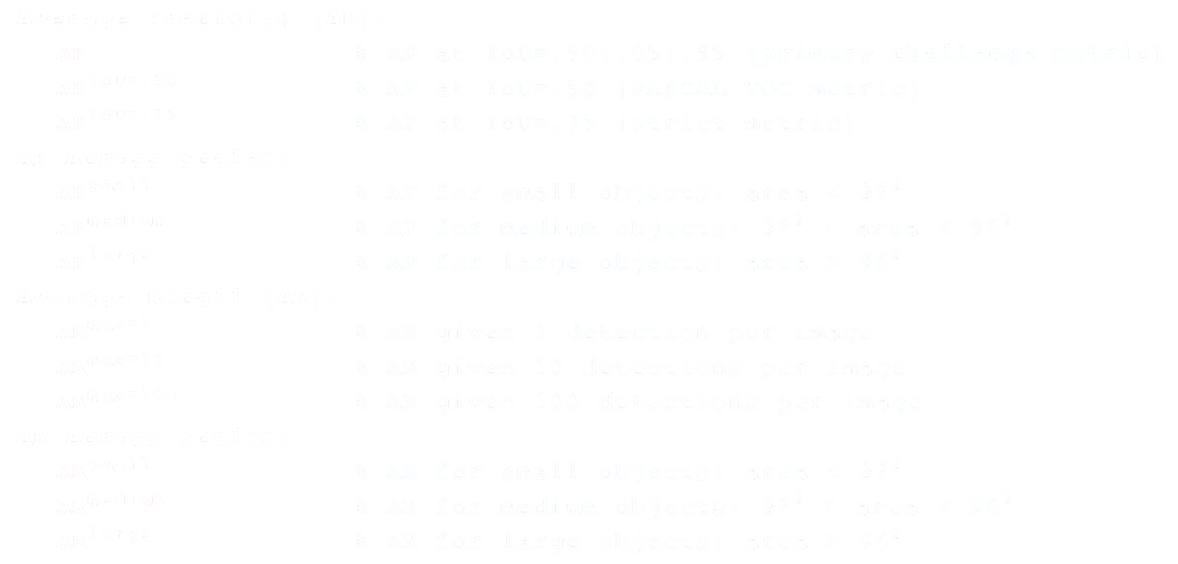
In the COCO competition, a total of 12 metrics are used to evaluate a model with the primary metric being mAP, which COCO refers to as AP, see table 12. One downside of the way AP was calculated in PASCAL is that it does not distinguish between how well a model localizes an object. As long as it achieves an IoU of more than \(0.5\), the object is considered correctly located. To incentivize more accurate localization, AP in COCO is averaged over \(10\) IoU thresholds in the range of \([0.5, 0.55, …, 0.95]\). The results are then averaged over all classes to get mAP, which is the primary evaluation metric.
In addition to mAP, there are specialized AP scores for objects of different sizes. These are defined by the amount of area an object covers in an image. We will later see why it is difficult for detectors to identify both large and small objects in images. So these scale related metrics help uncover weaknesses and strengths of particular models on this problem.
Moreover, averaged recall scores (AR) are reported as well. To get AR for a class you plot the recall of a model over different IoU thresholds in the range of \([0.5, …, 1]\) and take the area under this curve. The results are then averaged over all classes. This is useful since AR correlates strongly with localization accuracy for IoUs greater \(0.5\) [11]. Consequently, models with higher AR localize objects more accurately. Similar to AP, the performance for different scales are reported as well as the maximum recall when performing \(1\), \(10\) and \(100\) detection per image.
Overall, in the newer COCO competition, more distinct metrics are reported than in PASCAL which allows the evaluation of models on more criteria.
The future of benchmarks
While in COCO more metrics are reported than in PASCAL, the primary criteria to determine the winner is still the single metric: mAP. This one metric is used to evaluate how a given model performs on multiple different classes like animals and vehicles over a wide range of scales and view angles. By design, the results are general purpose object detectors which are tuned to detect objects from a wide range of classes well in images.
While in the earlier days the focus was on predicting the bounding box and associated class label correctly, with improvements in detectors, more distinct and refined metrics have been introduced like the mAP for objects of different sizes or AR, which reward greater localization accuracy. Moreover, these metrics can be used to figure out what types of objects and images the detectors perform poorly on.
Recently there is a debate on how useful these detection metrics still are for advancing the field. Since to perform well in a competition, mAP has to be high, other important aspects such as performance in the physical space, robustness against slight changes in the input through malicious adversarial attacks or the question of interpretability do not get the attention they require.
Now that we have an overview of how models are evaluated, we will see how some of them work starting with the more traditional object detection algorithms. Then we will give an overview of convolutional neural networks before diving into two popular and effective models: Faster R-CNN and YOLOv3.
References
[10] Everingham, M., Eslami, S. M. A., Van Gool, L., Williams, C. K. I., Winn, J., & Zisserman, A. (2015). The Pascal Visual Object Classes Challenge: A Retrospective. International Journal of Computer Vision, 111(1), 98–136. https://doi.org/10.1007/s11263-014-0733-5
[11] Hosang, J., Benenson, R., Dollár, P., & Schiele, B. (2016). What makes for effective detection proposals? IEEE Transactions on Pattern Analysis and Machine Intelligence, 38(4), 814–830. https://doi.org/10.1109/TPAMI.2015.2465908