Traditional Feature Extractors
What is a feature and why do we want to extract it from an image? Let’s say we want to detect the hollow cylinder in figure 5. Here, you can see that the contours are sufficient to describe the cylinder. These contours provide much more information than the uniform texture of the cylinder and consist of edges as well as a few corners. An edge is a sudden change in pixel intensity (brightness), whereas a corner is the intersection of two edges.
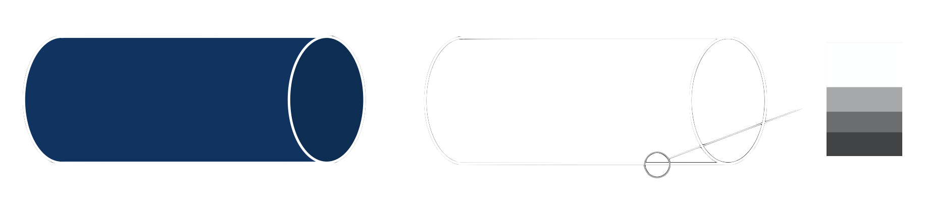
One major challenge in edge detection is visualized on the right of figure 5. The challenge lies in figuring out where this edge begins and ends when up close it looks more like a brightness gradient. This is traditionally determined by manually setting a threshold for the change in intensity, where noise has to be balanced with information loss. In practice, edge detection is often completed with the use of convolutions using fixed or manually tuned kernels, which are described in better detail under the section about convolutional neural networks.
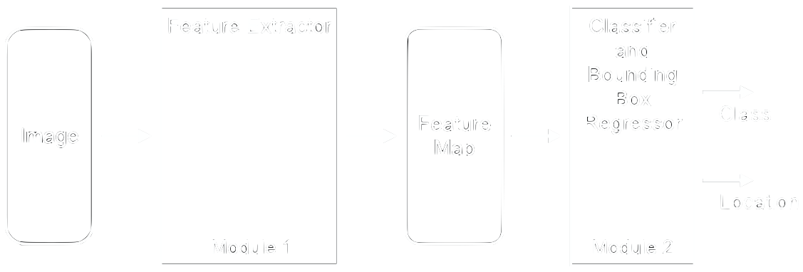
After obtaining the features, there are two principal ways to use them to recognize objects. One way is to match unique features from a new image with features of known objects directly. This is called keypoint matching where these unique features are known as keypoints. A second way is to use the feature map as an input for a classifier. The latter option has been shown to produce better results. Figure 6 shows the typical modules of object detectors as they were used from the mid 1990s to 2012.
Two of the most successful object detectors of their time are the Scale Invariant Features Transform (SIFT) [15] and Histograms of Oriented Gradients (HOG) [16]. Below we briefly introduce their principle ideas before we continue with the “modern” way: fully trainable convolutional neural networks.
Two Popular Feature Extractors: SIFT and HOG
The Scale-Invariant Feature Transform (SIFT)[15] and Histogram of Oriented Gradients (HOG)[16] are both popular traditional feature extractors that have competed in the ImageNet and PASCAL VOC competitions. SIFT looks at an image at different resolutions to make the computations scale-invariant, i.e. recognize objects regardless of whether they are far away or up close, to identify keypoints in the image. HOG, on the other hand, divides the image into a grid to create a grid of intensity gradients. Each grid cell would therefore have a distribution of intensity gradients, which can then be fed into a classifier.
Both the SIFT and HOG try to create features starting off with basic edge detection algorithms using fixed or manually tuned convolutions. Basic edge detection works by finding differences in pixel intensity compared to a pixel’s neighbours. These manually tuned convolutions extract the pixel intensity gradient and this gradient’s orientation, which are the basic features used for object detection.
The difference between SIFT and HOG is mainly in the way they structure the image for the calculations. SIFT uses consecutive downsamples of the image to create an image pyramid where each level represents the same image at a different resolution. At the smallest resolution, however, much information could have been lost from the downsampling. In order to preserve some of the lost information, the image is blurred using a Gaussian filter before being downsampled at each level. The Gaussian filter would, therefore, have passed over the image several times for the smallest resolution. This image pyramid represents the different scales acting on the image, thus allowing the algorithm to be scale-invariant.
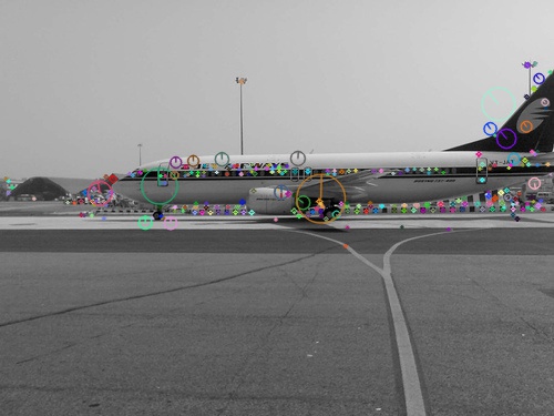
At each level of the image pyramid, the edge detection algorithm is used to find the gradient of pixel intensity and its orientation. A manually chosen threshold is then applied to the magnitudes of these gradients to create candidate keypoints. Keypoints in the same locations but on different levels of the image pyramid are combined with the keypoint with the largest magnitude gradient being selected. All of these keypoints can then be fed into a classifier, in which the original algorithm used a k-nearest neighbours to match the locations, magnitudes, and orientations to those of other known objects. Figure 7 shows an example of these keypoints on an airplane.
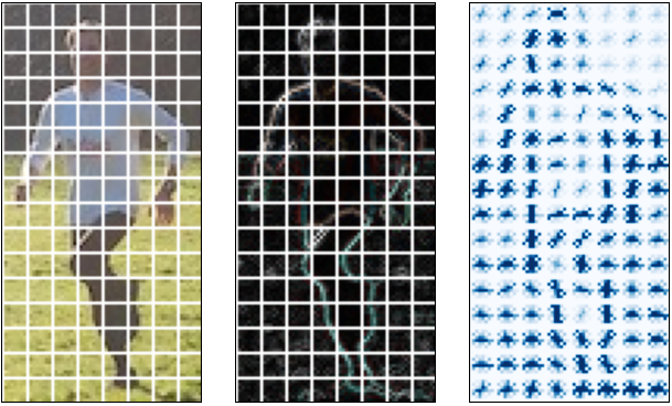
In contrast to SIFT, HOG divides the image into a grid rather than using a feature pyramid. You can see an example on the left side of figure 8. The gradient of pixel intensity is then calculated for each pixel within a grid cell (middle of figure 8). The orientations for each grid cell are then binned into discrete values (e.g. 0°, 20°, 40°, etc.) to suppress noise, creating a distribution or histogram of oriented gradients for each grid cell. Each bin would represent a discrete orientation increment with the height being the sum of the magnitudes of the gradient for each pixel within a grid cell. Then starting from the top left corner, the grid is normalized by grouping 4 grid cells and taking the average of the intensity gradient and dividing each grid cells’ values by this average. The grouping window then slides over one grid cell and this normalization operation is repeated throughout the entire image, creating a grid of oriented gradients (see example on the right of figure 8). These values can then be fed into a classifier, which originally used support vector machines.
The main advantage of using SIFT is that the image pyramid architecture allows it to create scale-invariant keypoint features. This image pyramid, however, is fairly computationally expensive. Conversely, HOG is not scale invariant and focuses on using the intensity gradient and orientation to be the features themselves. Though HOG is computationally faster than SIFT, it is not likely to be fast enough to be used in real time detection algorithms. Additionally, both of these algorithms have many different parameters that have to be manually tuned; thus, leading to the development of convolutional neural networks for object detection.
References
[15] Lowe, D. G. (2004). Distinctive Image Features from Scale-Invariant Keypoints. International Journal of Computer Vision, 60(2), 91–110. https://doi.org/10.1023/B:VISI.0000029664.99615.94
[16] Dalal, N., & Triggs, B. (2005). Histograms of Oriented Gradients for Human Detection. 2005 IEEE Computer Society Conference on Computer Vision and Pattern Recognition (CVPR’05), 1, 886–893. https://doi.org/10.1109/CVPR.2005.177