DeepFool
The DeepFool algorithm searches for an adversary with the smallest possible perturbation. The algorithm imagines the classifier’s decision space being divided by linear hyperplane boundaries that divide the decision to select different classes. It then tries to shift the image’s decision space location directly towards the closest decision boundary. However, the decision boundaries are often non-linear, so the algorithm completes the perturbation iteratively until it passes a decision boundary.
According to the authors this method generates very subtle perturbations in contrast to the coarse approximations of the optimal perturbation vectors generates by FGSM.
Figure 1 shows the concept behind DeepFool for a linear, binary classifier.
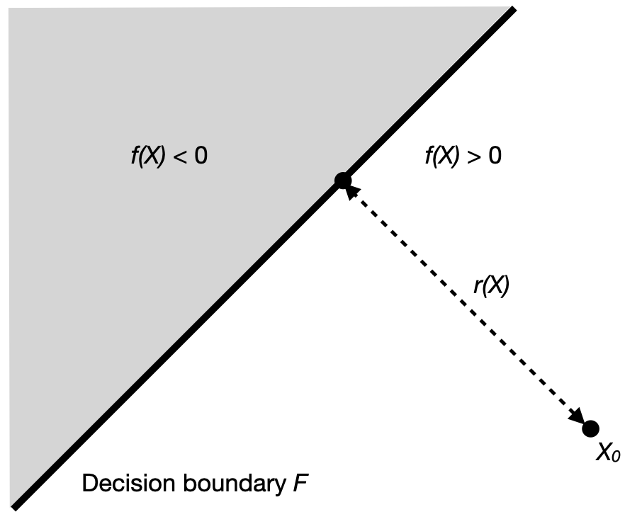
For an image \(X\) we get the minimum distance \(r_{min}\) to the decision boundary \(F\) by:
\begin{equation} \tag{4.1} r_{i}(X_{i}) = - \frac{F(X_{i})}{|| w ||_{2} } w \end{equation}
The algorithms uses equation 4.1 to generate an optimal perturbation \(r_{opt}\) in the following steps:
- Initialize the sample \(X_{0}\) with the clean image \(X\).
While \(sign( f(X_{i}) ) = sign( f(X_{0}) )\):
- Compute \(r_{i}\) with equation (4.1) and update
\begin{equation} \tag{4.2} X_{i+1} = X_{i} + r_{i} \end{equation}
Result: \(r_{opt}\)
For multi-class classifier the steps above can be generalized. For details see the original paper.
We use the Python implementation which is available from the authors and copy it to the modules folder.