Attacks
We now attack the model with the methods described in the implementation section and analyze their success. Along the way we develop and test hypothesis which apply to adversarial attacks.
The attacks are:
2.1 Fast Gradient Sign Method
The following is an example of the original image, the generated perturbance, and the resulting adversarial image using the Fast Gradient Sign Method:
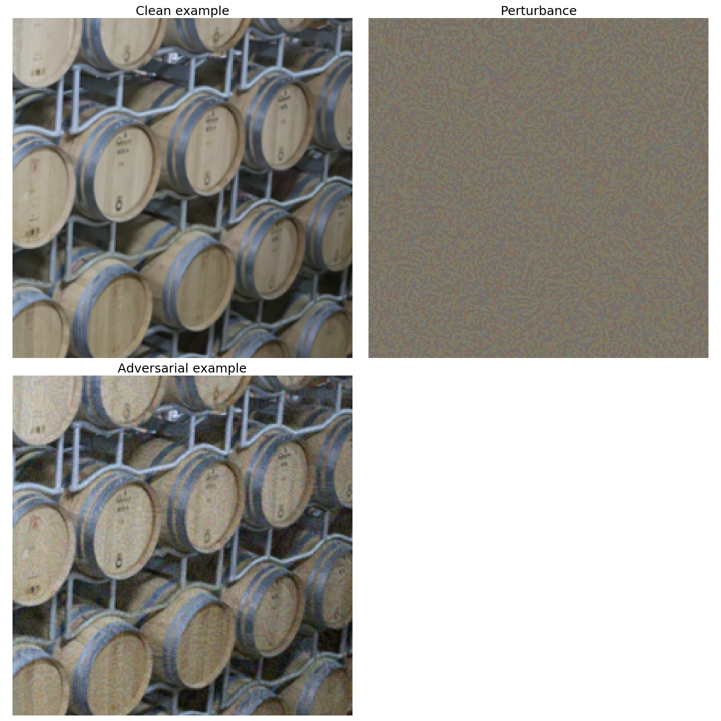
The adversarial image appears slightly blurrier than the original one, like for example taken at poorer resolution or with a worse camera. Without the reference image however, it can be difficult to tell that it has been modified. With increasing attack strength, this becomes noticeable as can be seen in the following images:
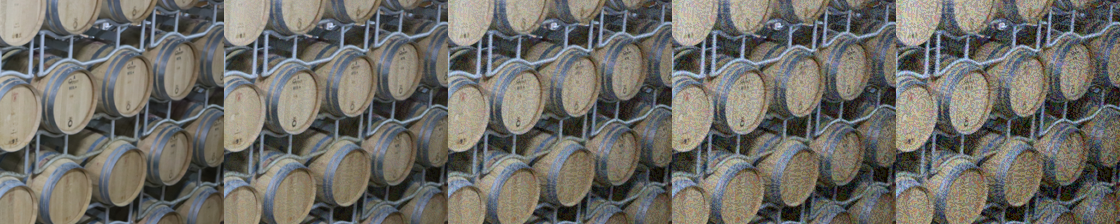
The image appears more and more noisy. We later show methods which produce cleaner looking adversaries.
But how effective is this attack in tricking the network? Recall that we want to produce images which cause a prediction of a wrong class at a high confidence. From figure 7 you can see that the confidence drops sharply while the class changes only for a few epsilons. The example above is the sample with which the model has one of the highest confidences on clean data. We have seen this same behaviour with other images with high confidence in the dataset. This leads us to the first hypothesis:
Hypothesis 1: Images with a high initial confidence are harder to manipulate.
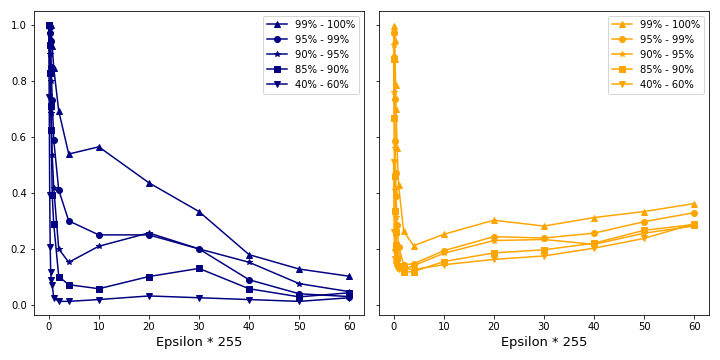
We consider a plot of accuracy and confidence over the attack strength epsilon in figure 5. For this hypothesis to be true we would observe a sharp drop in accuracy with increasing attack strength. The higher the initial confidence is, the smaller the slope of the accuracy should be. It is harder to attack the network at the same epsilon. At the same time the confidence should drop slightly since more and more robust features are altered.
Recall from the section Data Exploration how the confidence over all data is distributed. We consider correct initial classifications only and split the data into confidences ranges.
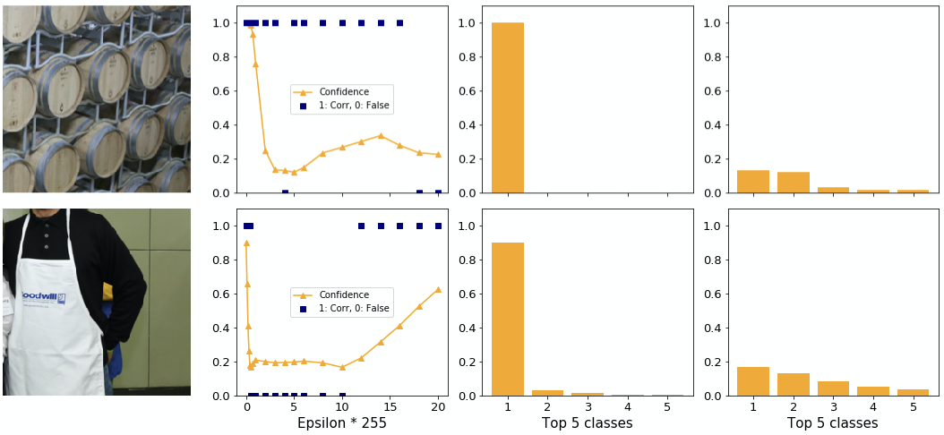
Observation: For FGSM, a stronger perturbance does not necessarily lead to more confident or successful adversaries.
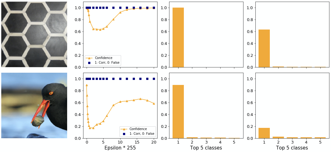
In theory, increasing the magnitude of the perturbation should lower the confidence of the model in predicting the correct class. We, however, have found some exceptions. Figure 6 shows two samples where the FGSM fails to attack. Interestingly, the confidence in the original correct class first drops quickly, then increases again with increasing adversarial perturbance. In the first example, the model’s confidence even reaches back to clean levels at the highest levels of perturbance.
A smaller increase in confidence after a dip can also be seen in figure 7. Despite the high initial confidence the adversary is able to change the class here. However, with a stronger attack the model predicts the correct class again. We found this behaviour of a bounce back to the correct class frequently for high initial confidences. Around the epsilon where the class changes we found that the highest and second highest confidences are very similar, whereas the gap to the third highest remains. The decrease in predictive confidence causes the second highest confidence to grow over proportionally which leads to the swap at the lowest point.
Observation: FGSM can craft adversaries with higher confidence than in the clean case for low confidence examples only.
The previous examples showed images with high initial confidence. It is not possible to generate an adversary with higher confidence than the original one for these cases. Figure 8 shows where it is possible. The initial confidence is quite low (around 50%). The FGSM can manipulate this image easily and achieves a confidence of 80%!
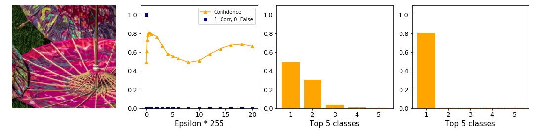
Observation: For FGSM the chance of an attack to succeed varies with each sample.
After analyzing the FGSM we now turn to a method derived from it, the basic iterative method BIM.
2.2 Basic Iterative Method
The authors in Adversarial Examples in the Physical World introduce BIM as an extension of FGSM to generate stronger adversaries for higher computational costs. In figure 9 we show the influence of the two hyperparameters \(\alpha\) and num_iter on the attack with the top image from figure 6. We see that BIM is able to generate an adversary which fools the network while FGSM cannot.
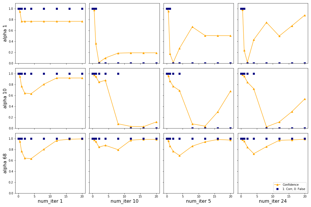
We can see that for this sample increasing \(\alpha\) generally causes the confidence to drop for smaller \(\epsilon\), as shown on the vertical axis from the top left corner. By increasing \(\alpha\) only it is not possible to change the predicted class. This is expected since \(\alpha\) is the parameter from the “fast” part of BIM and FGSM was not able to change the class for this image. However, changing the class is possible by increasing the number of iterations. The best results are in the top right plot (lowest \(\alpha\), highest number of iterations). For two \(\epsilon\) the networks predicts a false class with almost 80% confidence. Considering that FGSM was not able to change the class at all this is a strong result. The authors recommend keeping \(\alpha\) at 1/255 and changing the number of iterations with the heuristic shown in the section Implementation based on epsilon. For the remainder of this report we will choose these hyperparameters according to these recommendations.
In figure 10 we attack an image with high and low clean confidence, as we have done with FGSM in figure 7 and 8. In line with hypothesis 1 it is harder for BIM to manipulate the top image. However, while FGSM is able to change the predicted class for a few epsilons and at low confidence only, BIM is able to achieve an adversarial confidence of almost 80%. Moreover, the “bounce-back” effect seen with FGSM is not present here.
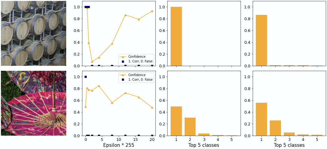
Interestingly, for the bottom image BIM is not able to generate higher confidence with the adversary. FGSM is working “sufficiently well” in this case. This leads us to the second hypothesis:
Hypothesis 2: For images with low initial confidence, FGSM’s ability to trick the network into predicting a false class is similar to BIM.
Given that in both cases the best adversary is for small epsilon it is likely that for both methods the perturbations are imperceptible. We investigate the perceptibility of adversaries generated by different methods in section 4 below.
The two methods analyzed so far generate untargeted attacks. Next, we investigate the ILLM which targets the least likeliest class. In the next section we will also analyze the performance of BIM further by looking at the general behaviour on all samples.
2.3 Least Likeliest Class Method
The ILLM method is related to BIM but is targeted by making the network predict the class with the lowest clean confidence, see section Implementation. Recall from figure 1 how for a well-trained classifier with a softmax output layer there generally is a significant gap between the highest and second highest confidence in the confidence distribution.
While BIM tries to increase the loss on the correct class, which then leads to the second class becoming more likely, ILLM tries to decrease the loss on the class with the lowest confidence (see minus sign in equation 3.2 from section Implementation/ILLM). We found that the result often is a low overall confidence as seen in figure 11. Note that ILLM is on average also less successful in attacking the model than the FGSM.
For future investigation it would be interesting to see how the order of the classes between the first (highest clean confidence) and last (lowest clean confidence) is effected by ILLM.
Observation: From the FGSM attack family, BIM produces the most successful and most confident adversaries.
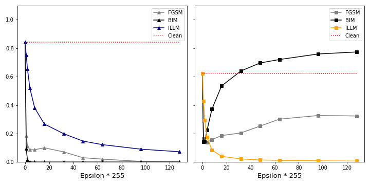
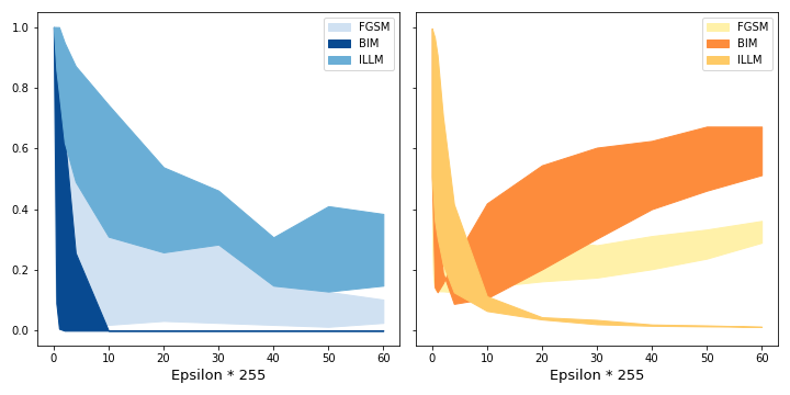
Figure 12 shows how the clean confidence influences the success of the crafted adversary. We see that hypothesis 1 applies. On the left side we see that for a given epsilon, the higher the clean confidence is, the fewer attacks are successful. We also see that there is a significant spread of the success of attack algorithms. It also shows how ILLM is least successful in attacking the model. On the right side we see how confident the generated attacks are. Adversaries generated with ILLM achieve the lowest confidences. The clean confidence only has a small effect. BIM on the other hand produces higher confident adversaries. Here, the spread is greatest.
How do individual examples behave? We find examples where ILLM performs poorly and well. In the top image of figure 13 the adversary tricks the network into believing it is looking at a hoop skirt rather than an apron. Considering that there are 1000 possible classes, including for example “baseball”, this choice seems poor since subjectively it is not very different. Additionally, the confidence is low. An adversary generated by BIM for example predicts “Arabian Camel” with 28% confidence.
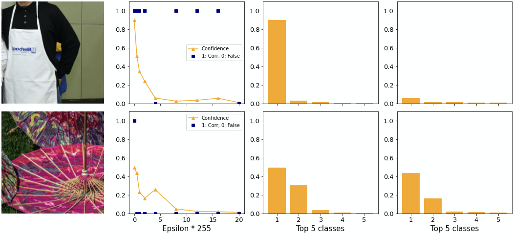
The confidence distribution in the top image is as expected relatively flat. It appears as if ILLM gives much more confidence to each class rather than concentrating the confidence on a few classes, as explained above.
Observation: ILLM does not consistently generate adversaries with very different classes from the original one. The cost of this attempt is a low adversarial confidence.
In the bottom image of figure 13 you can see another example. With the first epsilon the adversary is able to change the class to “lionfish”, the same as BIM does. However, as you can see on the rightmost plot, the confidence achieves over 80% adversarial confidence into same class. At the same time for ILLM the second class is higher than for BIM. This supports the notion that ILLM “flattens out” the confidence distribution rather than increasing the gap between 1st and 2nd.
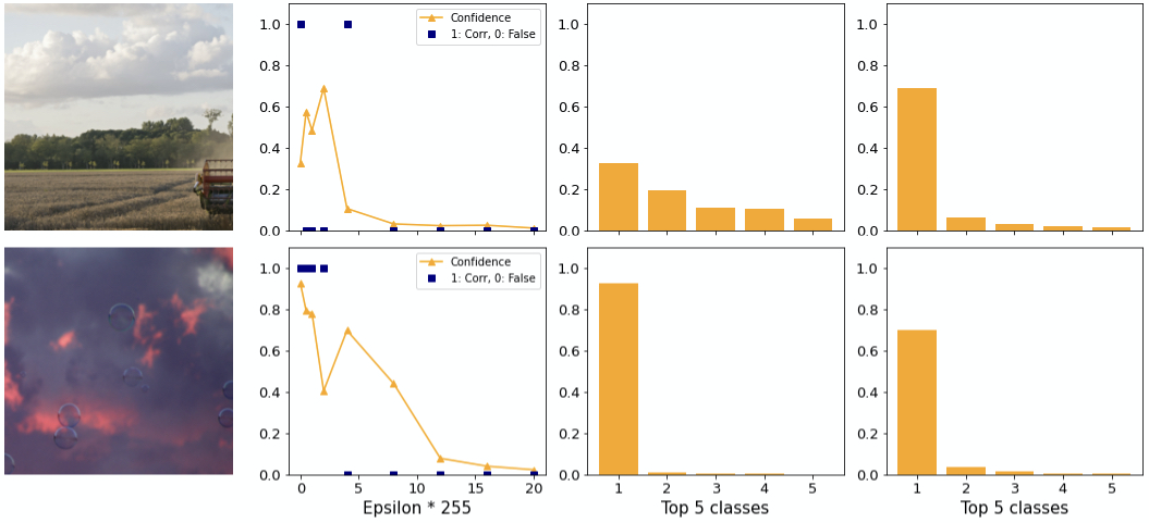
Two exceptions to this are shown in figure 14. On the top you can see a strong adversary with higher confidence than in the clean case. Here, the difference between first and second class is large. At the bottom image there is still a large difference. Note how hypothesis 1 applies. In both examples the confidence drops to close to 0 for greater epsilons.
In conclusion, we have found that BIM is sufficient for application not only to datasets with few classes but also to datasets with a lot of classes like ImageNet. In particular we found that ILLM does not consistently generate “interesting” examples (apron). Combined with the very low confidence of these adversaries and a similar perceptibility we did not find benefits of ILLM over BIM.
2.4 DeepFool
The methods which we have analyzed so far use the gradient to increase the loss which allows them to approximate the optimal perturbation. DeepFool finds the projected distance to the closest decision boundary and iteratively changes the adversary until the class has changed. The results are less perceptible adversaries.
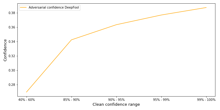
Figure 15 shows what influence the clean confidence has on the adversarial confidence for DeepFool. As expected for lower initial confidence the adversary achieves a lower adversarial confidence on average. The overall confidence of the adversaries is relatively low compared to BIM. DeepFool attacks are 100% successful and, as discussed in more detail in the next section, are always imperceptible.
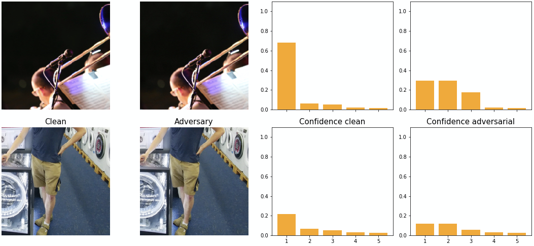
The effect DeepFool has on the network’s softmax output is illustrated in figure 16 on the example with the highest adversarial confidence (top). We can see how the confidences of adversarial class and the 2nd class in the softmax output are very similar. The same is true for the example with the lowest adversarial confidence (bottom). We have seen a similar distribution for other samples as well. We hypothesize that the reason for this is that DeepFool searches the closest decision boundary and slightly overshoots it.
In the next section we discuss the most interesting property of DeepFool, its imperceptible adversaries and compare them with adversaries generated by the other methods.