This section discusses the performance of the different adversarial attacks. First we briefly look at the properties of the clean data. Then we attack the model with different methods and analyze the success. We compare the perceptibility of adversaries generated by the different methods. Finally, we summarize our findings and point to future investigations.
1. Data ExplorationPermalink
Considering that the goal of adversarial examples is to fool the network into predicting a wrong class with high confidence, a good place to start start is to inspect the model’s performance without any adversarial perturbation.
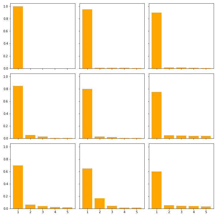
In the data there are 452 out of 1000 distinct classes represented. The most frequent class is ballplayer, baseball player (class index 981) with 8 occurrences, followed by racer, race car, racing car, stone wall and worm fence, snake fence, snake-rail fence, ... with 7 each. Within these frequent classes, the model’s confidence is around 58% with a standard deviation of around 27. This large range in confidence is likely due to false predictions. Figure 1 shows how the the top 5 confidence is distributed for different confidences in their top predictions.
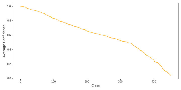
The average confidence for a class is between 99.99% (barrel, cask) and 41.64% (sandal). The distribution of the average confidence is shown in figure 2. For over half of the examples, the model has an average confidence of over 60% and over 23 of the examples have a confidence of over 50%.
The table shows the model’s overall performance.
| Confidence | Accuracy | |
|---|---|---|
| Top 1 | 0.69 | 0.84 |
| Top 5 | 0.63 | 0.97 |
Top 1 means that the predicted class is the correct class. Top 5 means that the correct class is among the 5 predicted classes with the highest score.