Feature Extractors Part 1 - Edge and Corner Detectors

This is the first of two parts about edge detectors and feature extractors before deep learning. In this part we will implement two basic extractors in Python with OpenCV.

Edges and corners are useful to detect objects in images. If you want to learn more about why we need these features and the basics of how they are calculated, see our section here. Today I want to focus on how to use common feature extractors in OpenCV. To follow along you can also get the repository.

Sobel filter

In an image, the interesting regions for feature extraction are regions where the pixel intensity changes. To detect the changes in intensity for a pixel, we compare its intensity with the adjacent pixels by sliding a small window in each direction. We then use a taylor series expansion to approximate the gradients of the pixel intensity in those directions.

The sobel filter implements this, along with a Gaussian smoothing operation.

To calculate this with OpenCV we first load an image:

import numpy as np
import cv2 as cv

img = cv.imread('images/pascal2007-plane.jpg')

In this example this is a colour image. To calculate the gradients for a colour image, OpenCV calculates the gradient for each colour channel and outputs the average. The calculation can be sped up by using a grey channel image instead, what we do next. We then convert the image into a numpy array.

# For performance we use a greyscale image
grey = cv.cvtColor(img, cv.COLOR_BGR2GRAY)
grey = np.float32(grey)

Now we calculate the gradients for the image grey. This is easy in OpenCV.

# Apply Sobel operator
ddepth = -1
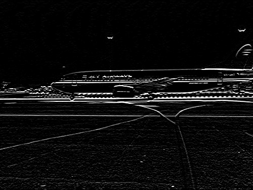
imgOut = cv.Sobel(grey, ddepth, 0, 1) # Gradients in y direction

Here, the second argument is the output image depth. In OpenCV depth is the precision of the pixel. A depth of \(-1\) yields the same depth as the input image. The third and fourth arguments indicate the directions of the derivatives. \((1,0)\) is the \(x\)-direction whereas \((0,1)\) is the \(y\)-direction. In Figure 1, we choose the \(y\)-direction for visualization since the fuselage of the airplane occupies most of the image which means there are a lot of horizontal edges.

Figure 1: Example for Sobel filter

And that’s already it! The intensity gradients can now be used for further tasks, like in the Harris corner detector.

Harris Corner Detector

The Harris filter, or corner detector, detects corners as the name suggests. Corners are interesting since they are small areas of the image which are generally invariant to translation, rotation and changes in illumination. Corners are used as features, for example, to stitch together multiple images to get a panorama or to detect objects.

The Harris filter detects corners in five steps. First, we convert the colour image into greyscale. Next, we search for the areas with a change in pixel intensity with a sliding window. Both of these first steps are similar to the Sobel filter. After some maths we end up with the following tensor which expresses the pixel intensity \(I\) derivatives in \(x\) and \(y\) direction

\begin{equation} M = \sum_{x,y} w(x,y) \begin{bmatrix} I_{x}I_{x} && I_{x}I_{y} \cr I_{y}I_{x} && I_{y}I_{y} \end{bmatrix} \end{equation}

where \(I_{x}\) is the first derivative of the x component into the \(x\) direction.

As the fourth step we get to the main part of the Harris detector. To determine if a sliding window position contains a corner, we use a score

\begin{equation} R = det(M) - k (trace(M))^2 \end{equation}

If \(R<0\) then there is an edge. If \(R\) is large then the area is a corner. Otherwise the region is flat.

In OpenCV we use

corners = cv.cornerHarris(grey, blockSize=2, ksize=3, k=0.04)

where grey is the input image, blockSize is the size of the neighbourhood from which the intensity is taken, ksize is the size of the kernel, and k is the parameter from the previous equation.

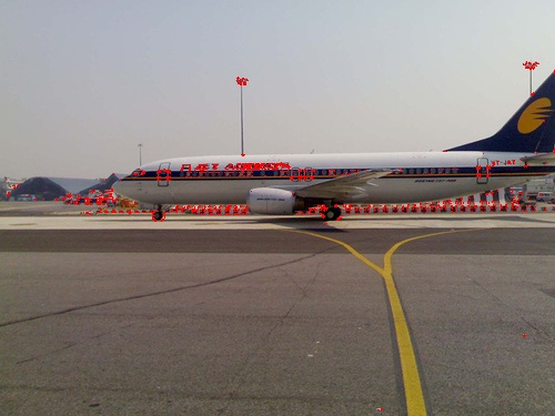
Figure 2 shows an example of Harris corners. As you would expect the corners on the windows are detected along with some other regions like the lights. To get better results, for example not missing any windows, the parameters can be adjusted.

Figure 2: Example for Harris corner detection

The full code for the example is:

import numpy as np
import cv2 as cv

img = cv.imread('images/pascal2007-plane.jpg')

# For performance we use a greyscale image
grey = cv.cvtColor(img, cv.COLOR_BGR2GRAY)
grey = np.float32(grey)

# Apply Harris operator
corners = cv.cornerHarris(grey, blockSize=2, ksize=3, k=0.04)

# Colour selected pixels where corners have been detected in red 
img[corners>0.01*corners.max()] = [0,0,255]

# Save image
cv.imwrite("images/harris-example.jpg", img)

# Show image with keypoints
cv.imshow('image', img)
cv.waitKey(0)
cv.destroyAllWindows()

We now know about two operators which are commonly used in traditional computer vision.