Feature Extractors Part 2 - SIFT and HOG
In the first part, we have looked at the Sobel filter which extracts approximations of pixel intensity gradients in images and the Harris filter to detect corners. Today, we will use two feature extractor which have been used successfully for object recognition: the Scale Invariant Feature Transform (SIFT) and Histogram of Oriented Gradients (HOG) in OpenCV. Both of them start with basic edge detection, similar to what we’ve seen in part 1. The code is available here. To learn more about how they work see this section.
SIFT
Scale Invariant Feature Transform is a feature extractor and object recognition pipeline which is built around using keypoints as features to detect objects regardless of scale.
To start, we load the image and convert it into greyscale.
1
2
3
4
5
import numpy as np
import cv2 as cv

img = cv.imread('images/pascal2007-plane.jpg')
grey = cv.cvtColor(img, cv.COLOR_BGR2GRAY)
Next we create a SIFT object.
1
2
# Create a SIFT object
sift = cv.xfeatures2d_SIFT.create(nfeatures=0, nOctaveLayers=3, contrastThreshold=0.09, edgeThreshold=10, sigma=1.6)
Here, we select the parameter values as in the paper. The first parameter, nfeatures determines how many of the best features to keep. A value of \(0\) keeps all keypoints.
The second parameter specifies the structure of the pyramid which is used. The pyramid consists of multiple downsamples (scales or octaves) and multiple Gaussian blurrings between each downsample. We can specify the latter here. In the paper, nOctaveLayers is \(3\). In OpenCV, we cannot select the number of octaves to use. They are calculated automatically from the image resolution.
The third parameter is used to filter out features in regions of low contrast. In these regions it is harder to distinguish an object from background. The greater this threshold, the fewer features will remain. In OpenCV this threshold is divided by nOctaveLayers when filtering is applied. Hence, we use \(0.09\) to work with the value from the paper, which is \(0.03\).
The next parameter, edgeThreshold is used to filter out edge-like features. These are features which are used to determine the boundaries between objects which is different from the contrastThreshold. The larger this threshold, the more features are retained. To understand the difference to the contrastThreshold, consider the image produced with the Sobel filter in part 1. Here, you can distinguish the plane from the tarmac by using the object boundaries only, not the contrast (since both plane and tarmac are black here by design). So both the edgeThreshold as well as the contrastThreshold could be considered as high.
The final parameter, sigma, is the \(\sigma\) used in the Gaussian blurring step which is applied at the first downsample in each octave. We use the default value \(1.6\).
Now that we have our sift object we can use it to identify and visualize the keypoints in the image.
1
2
3
# Detect and draw keypoints
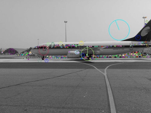
kp = sift.detect(grey, None)
img = cv.drawKeypoints(grey,kp,img,flags=cv.DRAW_MATCHES_FLAGS_DRAW_RICH_KEYPOINTS)
In figure 1, you can see the resulting keypoints as circles with the radius marked. The size of the circles indicate the magnitude while the line indicates the orientation of the keypoint. Interestingly, there’s an obviously not helpful keypoint of large magnitude above the plane.
Here is the full code:
1
2
3
4
5
6
7
8
9
10
11
12
13
14
15
16
17
18
19
20
import numpy as np
import cv2 as cv

img = cv.imread('images/pascal2007-plane.jpg')
grey = cv.cvtColor(img, cv.COLOR_BGR2GRAY)

# Create a SIFT object
sift = cv.xfeatures2d_SIFT.create(nfeatures=0, nOctaveLayers=3, contrastThreshold=0.09, edgeThreshold=10, sigma=1.6)

# Detect and draw keypoints
kp = sift.detect(grey, None)
img = cv.drawKeypoints(grey,kp,img,flags=cv.DRAW_MATCHES_FLAGS_DRAW_RICH_KEYPOINTS)

# Save images
cv.imwrite('images/sift-example.jpg', img)

# Show image with keypoints
cv.imshow('image', img)
cv.waitKey(0)
cv.destroyAllWindows()
HOG
Histogram of Oriented Gradients is a feature extraction pipeline which was first used to recognize pedestrians.
In OpenCV, the HOGDescriptor() function can be used to compute HOG features. However, the downside of the OpenCV implementation is that there is no simple way to visualize the features. That’s why we use scikit-image instead, which is a collection of image processing algorithms for Python specifically.
First, we load the image and normalize the pixel values so that they fall into the range \([0,1]\) as this is required for the skimage operations later. For this example, we use an image of size \(64x128\) as in the original implementation for pedestrian recognition.
1
2
3
# Read image
imgorg = cv.imread('images/pascal2007-person-correctsize.jpg') #  Use the correct size of 64x128 pixels
img = np.float32(imgorg) / 255.0
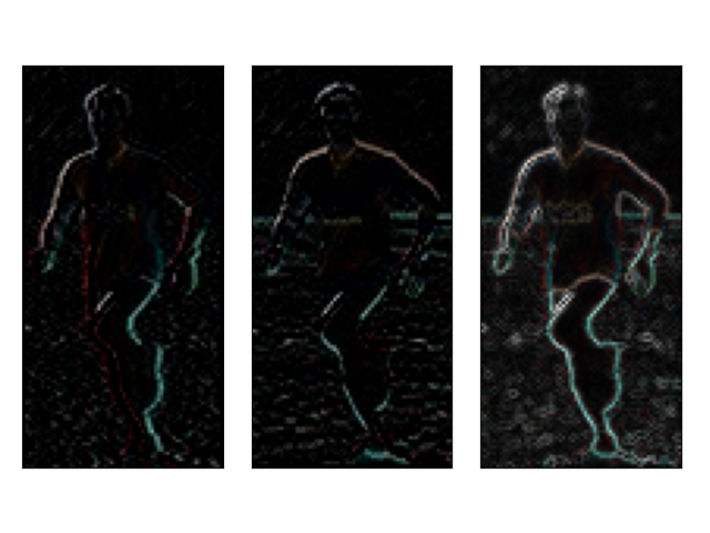
Next, we calculate the pixel intensity gradients for each pixel to find the magnitude and orientation for each gradient. We use the Sobel filter for this.
1
2
3
4
5
6
# Calculate gradient
gx = cv.Sobel(img, cv.CV_32F, 1, 0, ksize=1)
gy = cv.Sobel(img, cv.CV_32F, 0, 1, ksize=1)

# Find magnitude and orientation of gradients
mag, angle = cv.cartToPolar(gx, gy, angleInDegrees=True)
In figure 2, you can see the gradient magnitudes overlaid onto the image.
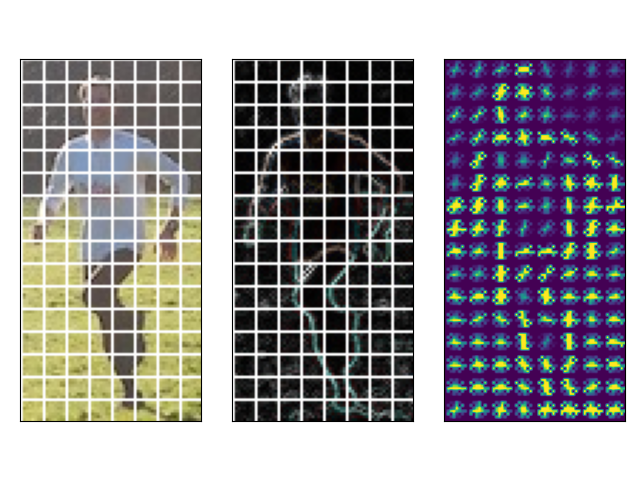
Once we have the gradients for each pixel we calculate the histograms for the grid cells on the image.
1
2
3
4
# Calculate HOG. Opencv doesn't offer visualization so skimage is used here.
implot = cv.cvtColor(imgorg, cv.COLOR_BGR2RGB)
fd, hogimage = hogsk(implot, visualize=True)
hogimage = exposure.rescale_intensity(hogimage, in_range=(0, 10))
The first part here changes the colour channel sequence from BGR as used in OpenCV to RGB as used in skimage and matplotlib. The third line calculates the HOG features, which are accessible as the first returned value fd. By selecting the visualization option in the second argument, the function also returns the image hogimage. For the visualization of the steps involved in HOG, we overlay the grid and get the result (figure 3).
And that is it. We now have the HOG features which can be used as input for a classifier for example.
Here is the full code:
1
2
3
4
5
6
7
8
9
10
11
12
13
14
15
16
17
18
19
20
21
22
23
24
25
26
27
28
29
30
31
32
33
34
35
36
37
38
39
40
41
42
43
44
45
46
47
48
49
50
51
52
53
54
55
56
57
import numpy as np
import cv2 as cv
from matplotlib import pyplot as plt
from skimage.feature import hog as hogsk
from skimage import data, exposure

# Read image
imgorg = cv.imread('images/pascal2007-person-correctsize.jpg') #  Use the correct size of 64x128 pixels
img = np.float32(imgorg) / 255.0

# Calculate gradient
gx = cv.Sobel(img, cv.CV_32F, 1, 0, ksize=1)
gy = cv.Sobel(img, cv.CV_32F, 0, 1, ksize=1)

# Find magnitude and orientation of gradients
mag, angle = cv.cartToPolar(gx, gy, angleInDegrees=True)

# Plot x, y, and magnitude of gradients
titles = ['Gradient x', 'Gradient y', 'Gradient magnitude']
for i in range(0,3):
    print(i)
    plt.subplot(1,3,i+1)
    plt.imshow(gx, cmap='Blues')
    plt.title(titles[i], color='white')
    plt.xticks([])
    plt.yticks([])
plt.tight_layout()
plt.savefig('images/hog-example-gradients.png', transparent=True)
plt.show()

# Calculate HOG. Opencv doesn't offer visualization so skimage is used here.
implot = cv.cvtColor(imgorg, cv.COLOR_BGR2RGB)
fd, hogimage = hogsk(implot, visualize=True)
hogimage = exposure.rescale_intensity(hogimage, in_range=(0, 10))

# Make grid 8x8 pixels for visualization
dx = 8
dy = 8
colour = [255, 255, 255]

implot[:,::dx,:] = colour
implot[::dy,:,:] = colour
mag[:,::dx,:] = colour
mag[::dy,:,:] = colour

titles = ['Original', 'Gradient magnitude', 'HOG feature map']
images = [implot, mag, hogimage]

for i in range(0,3):
    plt.subplot(1,3,i+1)
    plt.imshow(images[i])
    plt.title(titles[i], color='white')
    plt.xticks([])
    plt.yticks([])
plt.tight_layout()
plt.savefig('images/hog-example.png', transparent=True)
plt.show()