End-to-End Detection Transformer (DETR)
The Detection Transformer (DETR) model is a novel object detection model taking inspiration from the domain of natural language processing, namely transformers and attention [36]. As opposed to YOLO and Faster-RCNN architectures, DETR does not need to use non-max suppression or anchor boxes which have to be manually tuned. This streamlines the training pipeline compared to those other models because fewer hyperparameters need to be optimized.
Considering that the DETR model is based on the the multi-headed attention model described in the Attention is All You Need by Vaswani et al. [37], the reader should look into that for more details or this four part blog post [38]. A quick summary of multi-head attention is provided for those who just need a reminder of what it is or those who just want a brief overview.
Transformers Explained
Considering that the self-attention and transformers were originally used in the domain of natural language processing, this section will be explained in terms of natural language processing, i.e. the input to the model will be word sequences or sentences.
Normally, these words are mapped into their respective word embeddings which are vector representations of the properties of a word. This vector may contain a value to represent whether the word represents something that is edible, another may be its gender or whether it’s an animal. This creates an n-dimensional feature space where similar words are grouped close together while dissimilar words are far apart. For example, apple may be close to the words juice and orange while far from words such as car or newspaper. Note that these embedding values are normally obtained by training a model to do a simple task like filling in a missing word in a sentence found in literature, so it may be difficult to say which embedding value represents the word’s edibility and would likely be represented as some combination of embedding values.
What Is Attention?
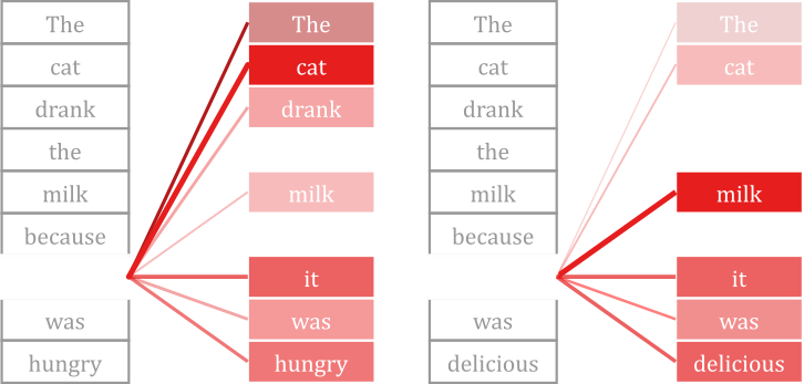
The idea of self-attention is based on figuring out how words in a sentence relate to the other words in a sentence. For example, in the sentence “The cat drank the milk because it was hungry”, the word “it” is referring to the word “cat”; whereas in the sentence “the cat drank the milk because it was delicious”, the word “it” is referring to “milk” despite the fact the only word that changed was “hungry” into “delicious” (fig. 34). Both sentences share identical grammatical structure and the changed words are both adjectives. However, we know what “it” is referring to from context and understanding that milk cannot be hungry and is presumably more delicious than a cat. Therefore, a self-attention model should create a high attention score between the words “cat” and “it” for the first sentence, while creating a high attention score between the words “milk” and “it” for the second one. This attention score allows the model to learn the relationship between words in a sentence, giving the model some contextual information and meaning. Transformers are a great tool for doing exactly that.
Transformer Overview
As can be seen in figure 35, the transformer is split into two main parts: the encoder (left) and the decoder (right). Starting from the bottom, a positional encoder is combined with the word embedding inputs with addition before being fed into the transformer. The encoder then alternates between using a multi-headed self-attention layer and a feed forward layer a number of times (normally 6) whose output is then fed into the decoder network. The decoder takes in a start token that is continuously concatenated with the most likely word from the output of the previous iteration, creating a loop. It then alternates between a multi-head self-attention layer, a multi-head attention layer integrating the encoder outputs, and a feed forward layer a number of times (normally 6). The feed forward layers in the network are simply fully connected layers with ReLU activation functions. As can be seen, the transformer is structured into residual blocks with skip connections. The decoder loop stops when it outputs an end of sequence or
The Positional Encoder
\begin{equation} \tag{1} PE_{pos, 2i} = sin(pos/10000^{2i/d_{model}}) \end{equation} \begin{equation} \tag{2} PE_{pos, 2i+1} = cos(pos/10000^{2i/d_{model}}) \end{equation} Where \(d_{model}\) is the word embedding length and i is the embedding position.
Normally, in recursive neural networks often used in natural language processing and in applications dealing with sequential data, inputs are fed into the network one by one so that the order of the sequence is implied by where each input was fed into the network. In self attention networks, they are fed into the network all at once and the order of the inputs does not matter. To encode the positional information of the sequence, a positional encoder consisting of sinusoids (eqs. 1 and 2) is added to the word embedding. The network would then be trained to learn that this sinusoid represents the position of the word [37].
The Self-Attention Layer
The self-attention layer first takes the input and multiplies it with three different trainable weight tensors to create key (K), query (Q), and value (V) tensors (fig. 36). There are several different types of attention formulas, but the one used in DETR and in [37] is the scaled dot-product attention:
\begin{equation} \tag{3} Attention(Q, K, V) = softmax \left(\frac{QK^{T}}{\sqrt{embedding\ length}}\right)V \end{equation}
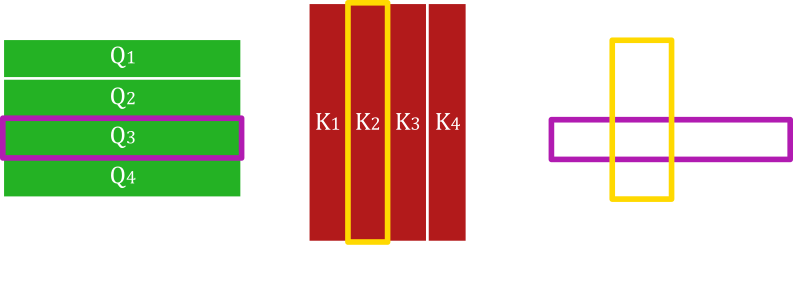
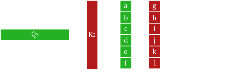
Overall, the scale dot-product* attention equation simply takes the value tensor and reweights it based on how similar words are between the query and key tensors. The key part of the equation is the QK^T which can be seen as the dot product between each word in the query and the key (fig. 37). A single word is represented as a row in the query tensor or a column in the transposed key tensor. The dot product works by multiplying each value in the query embedding with the respective value in the key embedding and summing them up (fig. 38). The denominator in the softmax function is used as a scaling factor to ensure that the result is within a certain range.
*If you are familiar with dot products from linear algebra, you may be familiar with using dot products to find the cosine similarity between two vectors. The dot-product between tensors simply expands this to find many different cosine similarities between the different vectors inside the tensors.
During the multiplication in fig. 38, if both values are positive or negative, the result is going to be positive or positively correlated. If only one value is positive and the other is negative, then the result will be negative. Finally, if one value is zero, then the product will be 0. All summed up, this gives in some sense how similar one word is to another (fig. 38).
The softmax function then takes negative values, representing dissimilar words, and outputs a number close to zero. Positive values, or similar words, has the softmax function output a number close to 1. The result of the softmax function is then multiplied with the value tensor to give the output of the self-attention layer.
In the decoder, you can find attention layers where the query, key, and values aren’t taken from the same source, but rather only the key and value tensors are taken from the encoder whereas the query tensor is taken from the previous decoder layer. The attention layer otherwise works exactly the same way, only with that slight modification in inputs. This integrates the information from the encoder into the decoder, i.e. it asks the question “how do the words in the input word sequence relate to the words that have been outputted so far”.
Multi-head attention
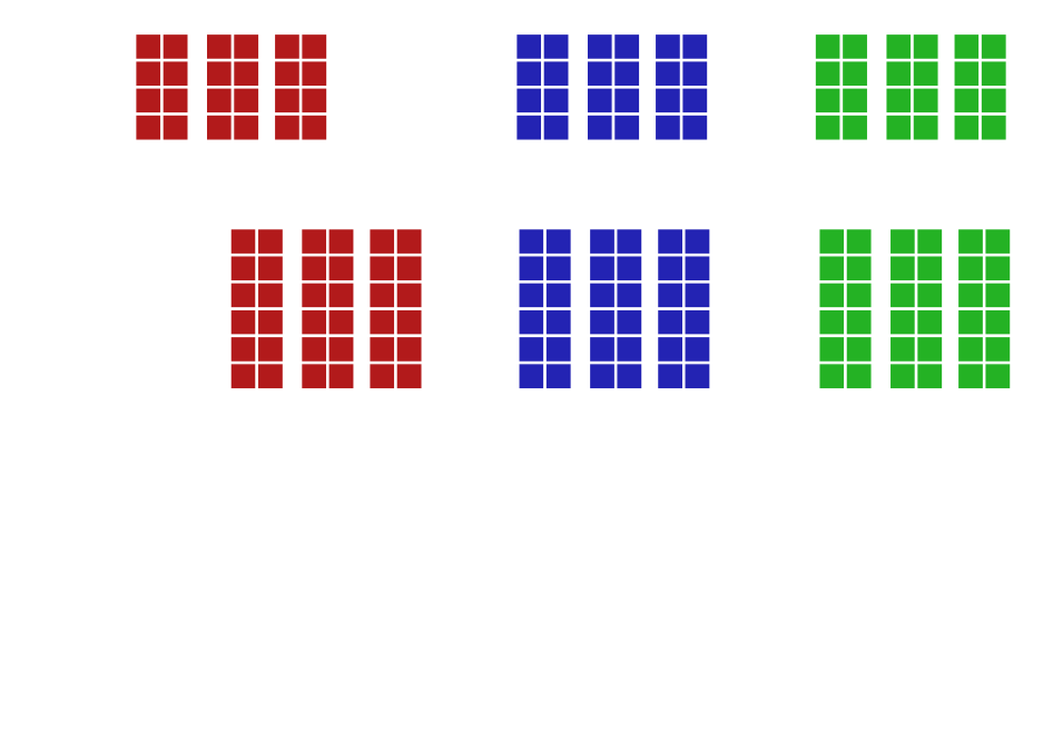
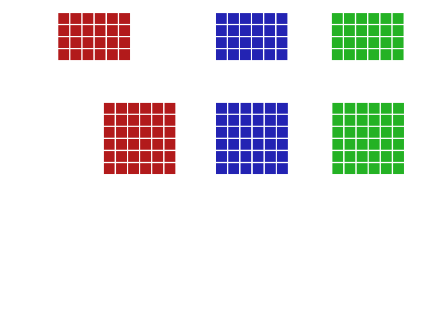
Multi-head attention is a simple optimization that seems to be able to increase the performance of a model without a significant increase in computational cost. The multi-head attention layer simply splits the weight matrices for each the query, key, and value tensors as can be seen in fig. 39. Note that although each piece of the entire key, value, or query tensor is split, each piece is calculated using the entire input tensor. Each query, key, and value tensor grouping is then fed into separate attention heads where each scaled-dot product operation is completed in parallel. All of the outputs are then concatenated together to create a single tensor of the same shape as the input tensor. It should be noted that the number of operations is not increased using multi-head attention, thus not increasing the computational cost.
What Does This Have to Do With Object Detection?
With a couple of small adjustments to the transformer model used in natural language processing, the transformer may be used for computer vision as well (fig. 40). First in the DETR model, the image is fed into a CNN such as ResNet-50. A positional encoding, similar to one used for natural language processing, is added to the output and then fed into the transformer system to encode the x and y coordinates of the image.
There are, however, no words or word embeddings in an image. Instead, each pixel is fed into the transformer like a word, and each pixel’s features act like its respective word embedding. The encoder then acts the same way as it did in natural language processing.
As for the decoder, it does not make sense to start off its input with a start token. In fact, object detection does not need to detect objects in sequence, so there is no need to continuously concatenate the output to the next input in the decoder. Instead, a fixed number of trainable inputs (in DETR, 100) are used for the decoder called object queries. Each of these object queries can be thought of as a single question on whether an object is in a certain region. This also means that each object query represents how many objects that the model can detect. Each of the decoder’s outputs are then fed into a fully connected network which is used as a classifier to determine what the object is.
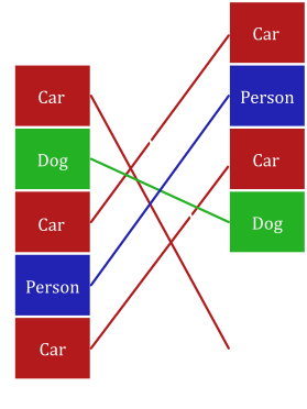
With the model always outputting a fixed number of object labels, many of the object labels need to be classified as “No Object”. Additionally, these objects could be in any order because any of the object queries could detect a specific object. Therefore, when training the model, the labelled data is padded with “No Object” labels to match with the size of the model’s output. A bipartite matching algorithm is then used to match each object with their respective true value. The matching algorithm completes the matching by minimizing the loss due to mismatched or poorly localized objects. If there is a mismatch in objects, the algorithm is forced to match predictions that are not the same as the label, penalizing the model loss greatly (fig. 41). Extra object predictions will be forced to match with “No Object” labels. The model, therefore, directly learns to predict the correct number of objects, so there is no need to use non-max suppression.
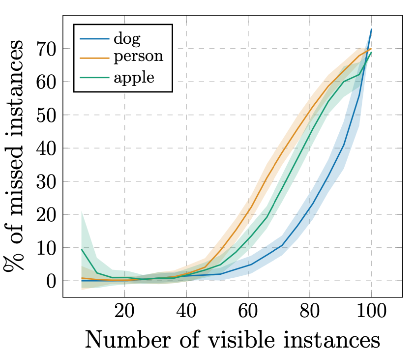
Because the model creates a fixed number of object labels, there is a hard limit on how many distinct objects DETR can detect. As you can imagine, the more objects there are to detect, the more likely an object will be missed. This is shown in fig. 42, where the percentage of missed instances starts to increase around the 50 objects mark. If it is expected that there will be too many object instances, the number of object queries can be increased at the cost of extra computational time.
Panoptic Detection
Similar to Mask-RCNN, DETR may be extended to complete panoptic segmentation by adding a simple mask head to each of its output (fig. 43). The data from the multi-head transformers is first reshaped back into its two-dimensional form. A mask head is added consisting of convolutional and upsampling layers to create mask-logits () for each object. To incorporate higher resolution information, in each upsampling operation, the model takes data from the convnet backbone at different resolutions and adds them in their respective resolution in the upsampling stages of the mask head. This is similar in style to a feature pyramid network which was covered in the YOLOv3 page. Finally, an argmax layer is then used to combine all of the masks together to segment the image into different classes. The result is that the image is then segmented pixel by pixel by simply using the most likely object class.
Performance
| \(Model\) | \(GFLOPS/FPS\) | \(\#params\) | \(AP\) | \(AP_{50}\) | \(AP_{75}\) | \(AP_{S}\) | \(AP_{M}\) | \(AP_{L}\) |
|---|---|---|---|---|---|---|---|---|
| FasterRCNN-DC5 | 320/16 | 166M | 39.0 | 60.5 | 42.3 | 21.4 | 43.5 | 52.5 |
| FasterRCNN-FPN | 180/26 | 42M | 40.2 | 61.0 | 43.8 | 24.2 | 43.5 | 52.0 |
| FasterRCNN-R101-FPN | 246/20 | 60M | 42.0 | 62.5 | 45.9 | 25.2 | 45.6 | 54.6 |
| FasterRCNN-DC5+ | 320/16 | 166M | 41.1 | 61.4 | 44.3 | 22.9 | 45.9 | 55.0 |
| FasterRCNN-FPN+ | 180/26 | 42M | 42.0 | 62.1 | 45.5 | 26.6 | 45.4 | 53.4 |
| FasterRCNN-R101-FPN+ | 246/20 | 60M | 44.0 | 63.9 | 47.8 | 27.2 | 48.1 | 56.0 |
| DETR | 86/28 | 41M | 42.0 | 62.4 | 44.2 | 20.5 | 45.8 | 61.1 |
| DETR-DC5 | 187/12 | 41M | 43.3 | 63.1 | 45.9 | 22.5 | 47.3 | 61.1 |
| DETR-R101 | 152/20 | 60M | 43.5 | 63.8 | 46.4 | 21.9 | 48.0 | 61.8 |
| DETR-DC5-R101 | 253/10 | 60M | 44.9 | 64.7 | 47.7 | 23.7 | 49.5 | 62.3 |
Table 4: DETR’s object localization performance on the COCO 2017 dataset using ResNet-50 and ResNet-101 backbones [36].
Based on the COCO 2017 dataset, the performance is comparable to that of an optimized heavily-tuned Faster RCNN model (table 4). Although DETR doesn’t detect smaller objects as well as Faster-RCNN, DETR is substantially better at detecting large objects. This is likely because it is processing global information over the entire image. Additionally, DETR runs at comparable speeds to that of Faster-RCNN.
| \(Model\) | \(Backbone\) | \(PQ\) | \(SQ\) | \(RQ\) | \(PQ^{th}\) | \(SQ^{th}\) | \(RQ^{th}\) | \(PQ^{st}\) | \(SQ^{st}\) | \(RQ^{st}\) | \(AP\) |
|---|---|---|---|---|---|---|---|---|---|---|---|
| PanopticFPN++ | R50 | 41.4 | 79.3 | 51.6 | 49.2 | 82.4 | 58.8 | 32.3 | 74.8 | 40.6 | 37.7 |
| UPSnet | R50 | 42.5 | 78.0 | 52.5 | 48.6 | 79.4 | 59.6 | 33.4 | 75.9 | 41.7 | 34.3 |
| UPSnet-M | R50 | 43.0 | 79.1 | 52.8 | 48.9 | 79.7 | 59.7 | 34.1 | 78.2 | 42.3 | 34.3 |
| PanopticFPN++ | R101 | 44.1 | 79.5 | 53.3 | 51.0 | 83.2 | 60.6 | 33.6 | 74.0 | 42.1 | 39.7 |
| DETR | R50 | 43.4 | 79.3 | 53.8 | 48.2 | 79.8 | 59.5 | 36.3 | 78.5 | 45.3 | 31.1 |
| DETR-DC5 | R50 | 44.6 | 79.8 | 55.0 | 49.4 | 80.5 | 60.6 | 37.3 | 78.7 | 46.5 | 31.9 |
| DETR-R101 | R101 | 45.1 | 79.9 | 55.5 | 50.5 | 80.9 | 61.7 | 37.0 | 78.5 | 46.0 | 33.0 |
Table 5: DETR’s panoptic segmentation performance on the COCO 2017 object segmentation dataset [36].
As can be seen in table 5, DETR is able to beat the other panoptic segmentation models in panoptic quality (PQ), segmentation quality (SQ), and recognition quality (RQ), despite using such a simple mask head. Additionally, it is able to perform that way despite the 7 point lead for PanopticFPN++ in AP.
Summary
DETR is a new object detection model that avoids using a lot of hand-crafted variables such as anchor box sizes and IoU thresholds used in non-max suppression. Rather it just asks the maximum number of objects it should expect in a single image. It is based on attention and can be extended to be used in panoptic segmentation and is fairly effective in detecting objects. Hopefully, there will be more work in using transformers in object detection that can improve DETR’s performance even further.
If you would like to check out DETR for yourself, you should go to the official DETR repo or our general object detector.
References
[36] Carion, N., Massa, F., Synnaeve, G., Usunier, N., Kirillov, A., & Zagoruyko, S. (2020). End-to-End Object Detection with Transformers. ArXiv:2005.12872 [Cs]. http://arxiv.org/abs/2005.12872
[37] Vaswani, A., Shazeer, N., Parmar, N., Uszkoreit, J., Jones, L., Gomez, A. N., Kaiser, L., & Polosukhin, I. (2017). Attention Is All You Need. ArXiv:1706.03762 [Cs]. http://arxiv.org/abs/1706.03762
[38] Doshi, K. (2020, December 13). Transformers Explained Visually. https://towardsdatascience.com/transformers-explained-visually-part-1-overview-of-functionality-95a6dd460452