You Only Look Once (YOLO)

The Faster R-CNN algorithm, while accurate, is fairly computationally intensive and is therefore not fast and light enough to be used for real time detection, especially on embedded devices. Instead of having a separate regions proposal stage, one-stage algorithms choose to forgo this initial stage and predict bounding boxes with class labels in one step. This section will therefore be describing YOLOv3 as an example of one of these one-stage detectors.

The You Only Look Once (YOLO) algorithm is a popular real-time capable object detection algorithm originally developed in 2016 by Redmon et al.[27]. Since then, it has been tweaked to increase its speed and localization performance. The main benefit of YOLO over Faster R-CNN is that it is several times faster than Faster-RCNN, while maintaining similar mAP scores, a measure of object localization performance. We will be mainly referring to YOLOv3 [28], introduced in 2018 as the most recent version developed by Joseph Redmon and Ali Farhadi.

Figure 26. General Architecture of YOLOv3.

YOLOv3 mainly consists of two parts (figure 26): a feature extractor and a detector. The image is first fed into the feature extractor, a convolutional neural network called Darknet-53. Darknet-53 processes the image and creates feature maps at three different scales. The feature maps at each scale are then fed into separate branches of a detector. The detector’s job is to process the multiple feature maps at different scales to create grids of outputs consisting of objectness scores, bounding boxes, and class confidences. The next section goes into further detail about the architecture starting with Darknet-53.

Darknet-53

The first part of YOLOv3 is the feature extractor: Darknet-53 (figure 27). It uses 53 convolutional layers, so this version is referred to as Darknet-53 as opposed to the much smaller Darknet-19 used in YOLOv2. With so many layers, the feature extractor needs to use residual blocks to mitigate the vanishing gradient problem. The Darknet feature extractor, therefore, mainly consists of convolutional layers grouped together in residual blocks alternating between \(3x3\) and \(1x1\) convolutional layers. Instead of using max pooling or average pooling layers to downsample the feature map, Darknet-53 uses convolutional layers with strides of \(2\) which skips every other output to halve the resolution of the feature map. Additionally, batch normalization is used throughout the network to stabilize and speed up training while also regularizing the model.

The end portion of the network is only used when YOLOv3 is used as a classifier rather than for object detection. For object detection, three outputs at different feature resolutions (in this case \(32x32\), \(16x16\), and \(8x8\)) to be fed into the detector. These outputs come from the last residual block at a specific resolution which would have the most complex features. These three outputs allow for multi-scale detection, i.e. detecting large and small objects, which will be described in more detail in the next section.

Multiscale Predictions

Localizing objects of vastly different sizes in an image can be difficult. Although creating deeper and deeper layers leads to more complex features, the repeated downsampling of the feature map may lose some of the finer details when making predictions. The output created at the end of the feature extractor may be too low of a resolution to precisely predict a bounding box around an object, particularly small ones. To compensate for this lack of resolution, the network can also use higher resolution feature maps from earlier layers to create separate predictions.

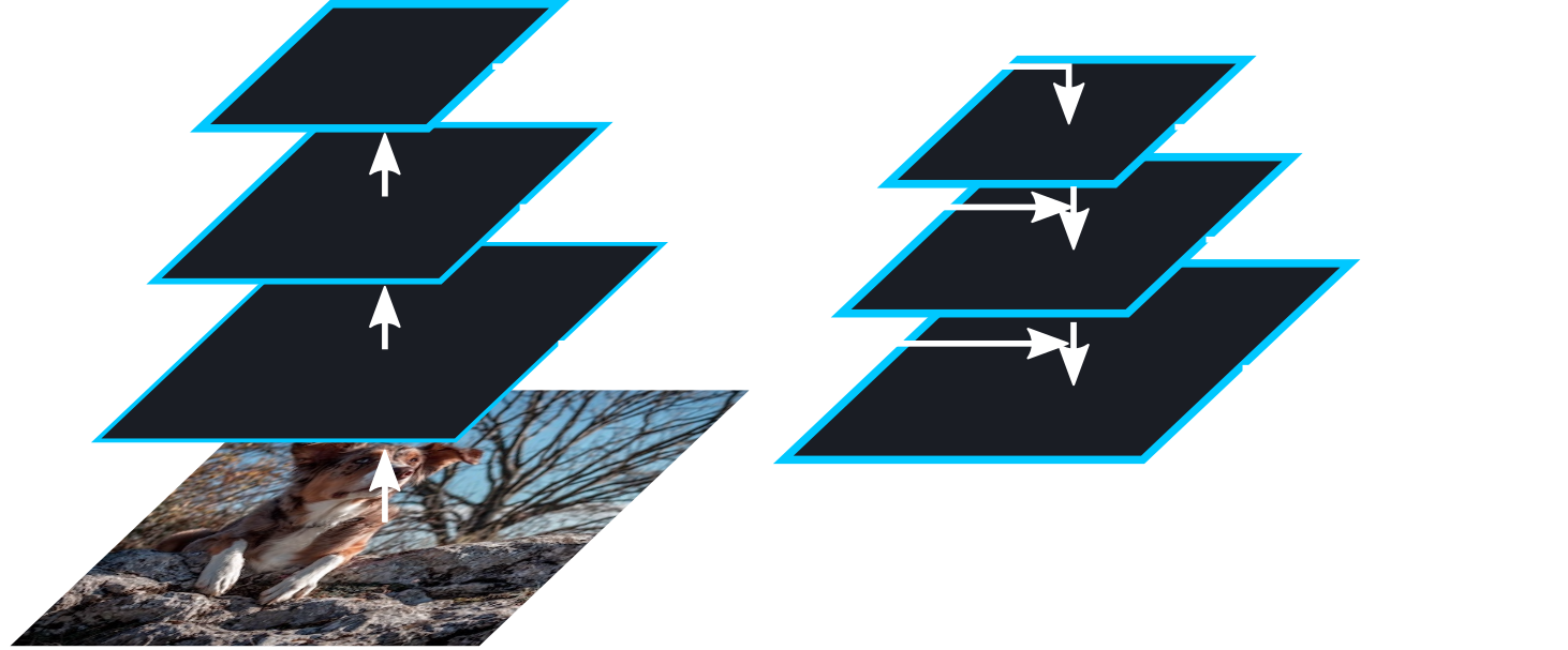
Figure 28. A feature pyramid network similar to one found in YOLOv3. Adapted from [29].

YOLOv3 makes use of a pyramid architecture similar to that of a feature pyramid network (figure 28) which was originally inspired by the multiscale predictions done in traditional feature extractors such as SIFT. In YOLOv3, the Darknet-53 feature extractor outputs three feature maps at three different resolutions. Each of these feature maps are then fed into the detector to make three separate prediction grids. The idea is that by using three different resolutions, the model will hopefully be able to identify objects at different scales, making the model more scale-invariant.

Figure 29. The YOLOv3 detector network including multiscale predictions. The number of grid cells at the smallest scale was chosen arbitrarily as 8x8. Adapted from [30].

The YOLOv3 detector part of the model mostly consists of three streams of convolutional layers in parallel: one for each feature map at each spatial resolution (figure 29). The lower resolution feature maps, however, tend to have more complex features while the higher resolution features have simpler features. YOLOv3, therefore, successively upsamples and then concatenates the lower resolution features with the next higher resolution map. This allows the higher resolution feature maps to make use of the more complex features found at lower resolutions.

The detector then outputs three separate outputs at different resolutions: a small scale, medium scale, and large scale output. These outputs divide the image into differently sized grid cells and each grid cell contains multiple anchor boxes. How these grid cells are formed will be described in the next section.

Grid Cells

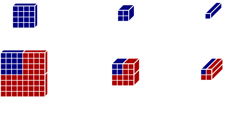
YOLOv3 divides the input image into grid cells where if an object’s centrepoint lands on a particular grid cell, that grid cell will be responsible for detecting it with its three (or more) anchor boxes. These grid cells arise from the architecture of Darknet-53, which is illustrated in a simplified example in figure 30. In figure 30 top, the input is reduced from a \(4x4\) to a \(1x1\) resolution. The same operations acting on an \(8x8\) input creates a \(2x2\) output (figure 30 bottom). Each component of this output then represents a grid cell of the input image.

The size of the grid cell is only based on the downsampling operations (e.g. max pooling) in the neural network. In Darknet-53, the 5 downsampling steps that halve the resolution making the grid cells \(32\) pixels wide at the lowest resolution feature map, forcing the input image to have a resolution of a multiple of \(32\). Larger images simply have more grid cells, so a \(480x320\) pixel image would have \(15x10\) grid cells at the coarsest grid cell resolution. Images that do not have resolutions of multiples of \(32\) pixels can be preprocessed by being cropped, stretched, or padded to meet this criterion or resized to keep the network small and fast.

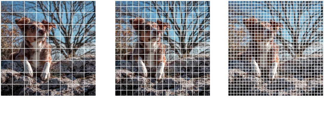
Figure 31. Grid cells used in YOLOv3 for multiscale predictions.

With multi-scale predictions, YOLOv3 creates three different sets of grid cells for each scale (Figure 31). Many of these grid cells will overlap and each scale will specialize in different object sizes. The small scale output has smaller anchor boxes to handle smaller objects while the larger grid cells use much larger anchor boxes to handle larger objects. This allows YOLOv3 to detect objects of vastly different sizes.

It should be noted that although each grid cell acts like an input, the output looks at a much wider area of the picture because each convolution also looks at values neighbouring the grid cell. For example, the right most 3x3 convolution of a grid cell will look at values from the grid cell to the right. Considering that Darknet-53 has 53 convolutional layers, many of them \(3x3\) convolutions, each grid cell takes in information from large areas of the input image, if not the entire image.

The Output

Finally, after talking so much about how YOLOv3 works, we can talk about YOLOv3’s output. YOLOv3’s output consists of three grids of outputs, one for each scale resolution (figure 31). The image is divided so that each grid cell is only responsible for detecting an object when the object’s centre lands within that particular grid cell.

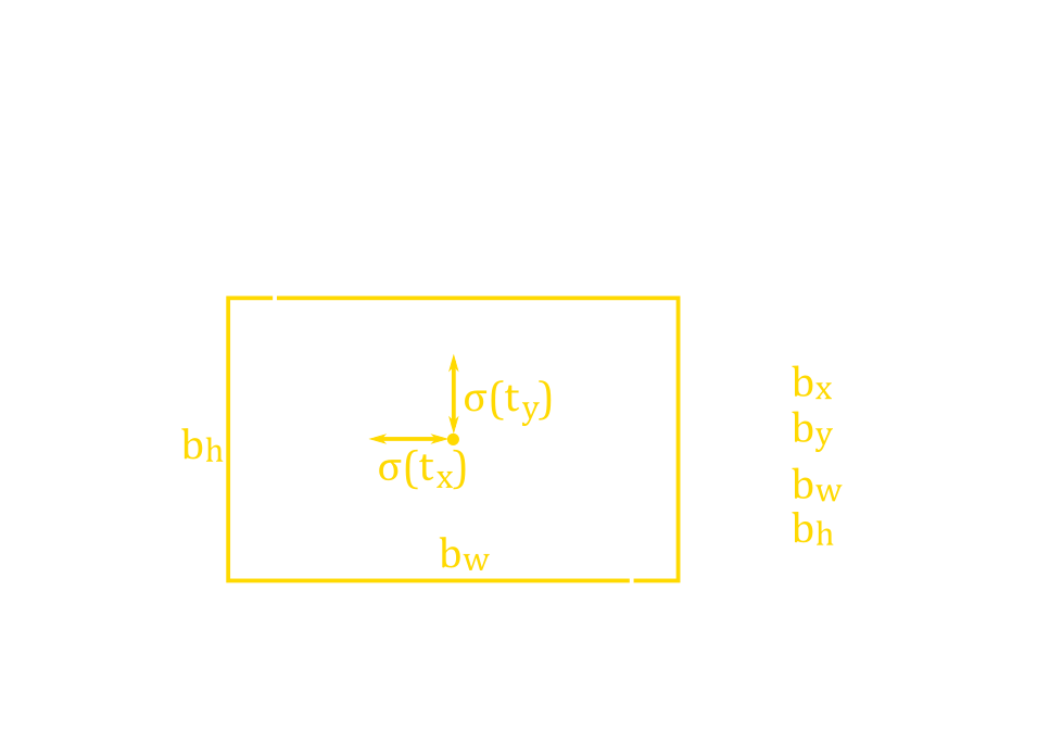
Like Faster R-CNN, YOLOv3 uses anchor boxes where each grid cell contains three anchor boxes each. The output for each anchor box then consists of \(4\) variables to represent the size and location of the bounding box within the cell (tx, ty, tw, and th), an objectness score similar to that used in Faster R-CNN, and a number of class confidence scores. This means the output size for each grid cell is (number of anchor boxes)*(1+4+number of classes).

The bounding box coordinates are made relative to the centre of the grid cell and the original size of the anchor box (figure 32). Although these anchor boxes are later refined, it would be easier for the network if these anchor boxes were already close to the objects’ dimensions. So, a K-means clustering algorithm was used on the training dataset to find a set of anchor box dimensions that can fit a wide variety of objects. These anchor box dimensions are then divided across the different resolutions. The user can also adjust the number of anchor boxes if they would like the anchor boxes to cover more dimensions.

Figure 32. Bounding boxes with dimensions and priors locations. Adapted from [31].

With three bounding boxes predicted per grid cell at three different spatial resolutions, hundreds of bounding boxes are predicted. Considering that an image likely only has a handful of objects, many of these bounding boxes will have to be removed. The objectness score is used to threshold the existence of the object, so bounding boxes with less than \(0.5\) objectness scores are removed. Multiple bounding boxes will still likely exist for the same object, so non-max suppression is used to remove bounding boxes predicting the same class and have high overlap (IoU) with each other, keeping the ones with the highest confidence.

When making the class confidence scores, Redmon chose to use independent logistic classifiers rather than the usual softmax function. Using independent logistic classifiers allows for multilabel classification in case there are overlapping class labels (e.g. an husky is both a dog and a mammal). Redmon found it unnecessary to use a softmax function for good performance; although it is simple enough to change if there are no overlapping labels.

Strengths and Weaknesses

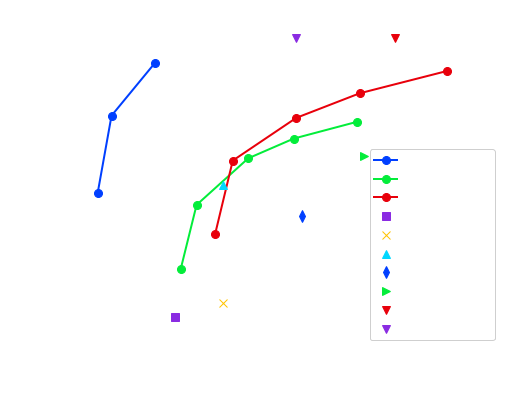
Figure 33. mAP vs. model speed of various object detection algorithms using the COCO dataset with IoU=0.5 threshold. Data taken from [32] and [27].

The main strength of YOLOv3 is that it can run fairly quickly while maintaining a competitive localization accuracy (Figure 33). The model is light enough that it can run on embedded systems or mobile devices. YOLOv3 is even fast enough for real time detection which is normally benchmarked to be \(30\)fps or \(33\)ms. This speed is mainly because YOLOv3 completes almost everything at once and requires only one forward pass. Additionally, it generalizes fairly well when, for example, the model is trained on real images and then later testing on objects depicted in art.

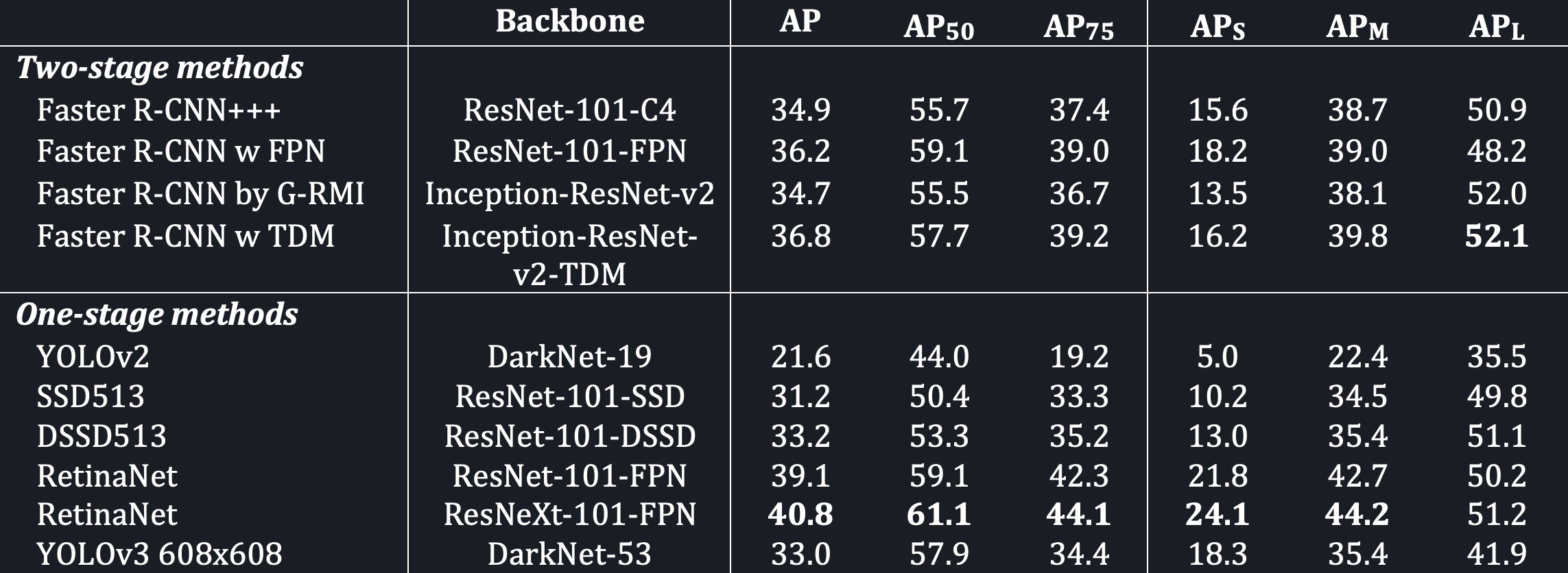
Table 3. Localization performances of different models on the COCO dataset. Taken from [28].

The drawbacks of YOLOv3 are that it is not the most accurate object localization algorithm. Figure 33 shows the performance of YOLOv3 on the COCO dataset where the IoU threshold is 0.5. If looking at the Average Precision where the IoU threshold is set to 0.75 (Table 3), YOLOv3 does much worse than Faster R-CNN. This means that YOLOv3 has trouble precisely placing the bounding box precisely around objects. Additionally, looking at the Average Precisions for medium and large objects (AP_M and AP_L), YOLOv3 does not seem to deal with medium or large sized objects very well relative to the other models. YOLOv3 sometimes also has problems with objects whose centres lie near the edge of grid cells. Finally, there does not seem to be a direct way to generalize the model for object segmentation tasks.

YOLOv3 is the last of the quick object localization models created by Joseph Redmon. This, however, is not the end for YOLO. In 2020, three new YOLO models were released by three different groups: YOLOv4 [33], YOLOv5 [34], and PP-YOLO [35]. All three of these models were built on the YOLOv3 implementation and have shown substantial improvements in localization accuracy, speed, or both. We hope that learning about YOLOv3 taught you about different techniques.

References

[27] Redmon, J., Divvala, S., Girshick, R., & Farhadi, A. (2016). You Only Look Once: Unified, Real-Time Object Detection. ArXiv:1506.02640 [Cs]. http://arxiv.org/abs/1506.02640

[28] Redmon, J., & Farhadi, A. (2018). YOLOv3: An Incremental Improvement. ArXiv:1804.02767 [Cs]. http://arxiv.org/abs/1804.02767

[29] Lin, T.-Y., Dollár, P., Girshick, R., He, K., Hariharan, B., & Belongie, S. (2017). Feature Pyramid Networks for Object Detection. ArXiv:1612.03144 [Cs]. http://arxiv.org/abs/1612.03144

[30] Li, E. Y. (2019, December 30). Dive Really Deep into YOLO v3: A Beginner’s Guide. https://towardsdatascience.com/dive-really-deep-into-yolo-v3-a-beginners-guide-9e3d2666280e

[31] Redmon, J., & Farhadi, A. (2016). YOLO9000: Better, Faster, Stronger. ArXiv:1612.08242 [Cs]. http://arxiv.org/abs/1612.08242

[32] Lin, T.-Y., Goyal, P., Girshick, R., He, K., & Dollár, P. (2018). Focal Loss for Dense Object Detection. ArXiv:1708.02002 [Cs]. http://arxiv.org/abs/1708.02002

[33] Bochkovskiy, A., Wang, C.-Y., & Liao, H.-Y. M. (2020). YOLOv4: Optimal Speed and Accuracy of Object Detection. ArXiv:2004.10934 [Cs, Eess]. http://arxiv.org/abs/2004.10934

[34] Jocher, G. (2020). YOLOv5. https://github.com/ultralytics/yolov5

[35] Long, X., Deng, K., Wang, G., Zhang, Y., Dang, Q., Gao, Y., Shen, H., Ren, J., Han, S., Ding, E., & Wen, S. (2020). PP-YOLO: An Effective and Efficient Implementation of Object Detector. ArXiv:2007.12099 [Cs]. http://arxiv.org/abs/2007.12099