Faster R-CNN
In the previous section, we introduced convolutional neural networks and explained how they can be used to classify objects. Object classification, however, is normally the simplest out of the object recognition tasks. In classification tasks, often only one object is in the image which is usually featured prominently at the centre.
Object detection, however, involves determining which areas of the image contain objects apart from the image background (e.g. grass and sky) in addition to classifying them. These objects’ locations are normally defined with boxes drawn around the object called bounding boxes, as shown in the introduction and in figure 19 right.
Faster Region Based Convolutional Neural Network (Faster R-CNN) [22] is one of the top models used for object detection. It is a two-stage object detector which was originally presented in 2015 as the third iteration of the R-CNN family of object detectors. It mainly consists of two modules: a first module to localize objects (called the region proposal module) and a second module to assign class labels to these objects (called the detector module), see figure 19.
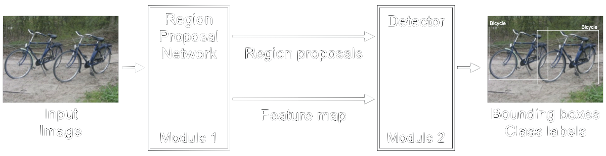
The region proposal module takes the input image and extracts features and region proposals. Region proposals are parts of the image which most likely contain an object. Each of these regions are then processed by the detector in which a multiclass classifier labels each region proposal, removing redundant proposals, and refines the bounding boxes via a regressor. Both of these modules utilize convolutional neural networks.
Faster R-CNN is available in Detectron2, the latest system for object detection from Facebook AI Research.
Module 1: Region Proposal Network
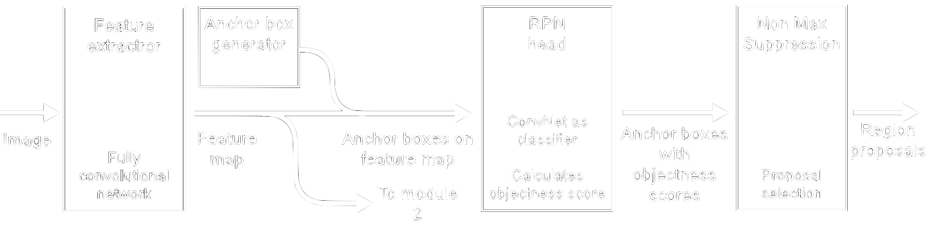
The Region Proposal Network (RPN) takes an image of any size as input and returns a map of convolutional features and regions of the image, which most likely contain objects (figure 20). The introduction of the RPN is one of the major changes to Faster R-CNN compared to its predecessor, Fast-RCNN [23], to tackle a computational bottleneck in its regions proposal algorithm [22]. While it is called a neural network, it should really be thought of as two neural networks, one to extract features and the other to calculate how likely a region of an image contains an object, plus a post-processing step to remove proposals that do not contain objects.
Base network - FCN for feature extraction
To create the region proposals, the first step is to use a fully convolutional network (FCN) [24] to extract features from the image. An FCN is a convolutional neural network without the fully connected layers and the softmax layer, which are used in convolutional neural networks for classification (see the section ConvNet Basics). This stops the network at the feature extraction step, creating a feature map similar to the original image except that instead of colour channels, it has feature channels. This feature map has dimensions \(W x H x ConvDepth\) (width, height and number of filters) which are fed into the RPN head to compute the objectness score. The original paper used a modified version of the VGG-16, which we explained in the previous section.
Anchor boxes for regions of interest
Now that we have the feature map we need to find a way to tell the RPN head where to look for objects. This is where anchor boxes come into play. Anchor boxes are bounding boxes which are placed over the whole feature map and serve as locations at which the RPN is going to search for objects.
To place those anchor boxes, the feature map is divided into a regular grid first, see figure 18. Next, we place a number of anchor boxes, centred on the centre of the cell, into each of these grid cells. It is up to us how many of those anchor boxes we choose and of what size and aspect ratio they are. These parameters should be tailored according to the objects which we aim to detect. In figure 19 we show two aspect ratios and three boxes as an example. For pedestrian detection for example, we would take boxes with \(width < height\) only.
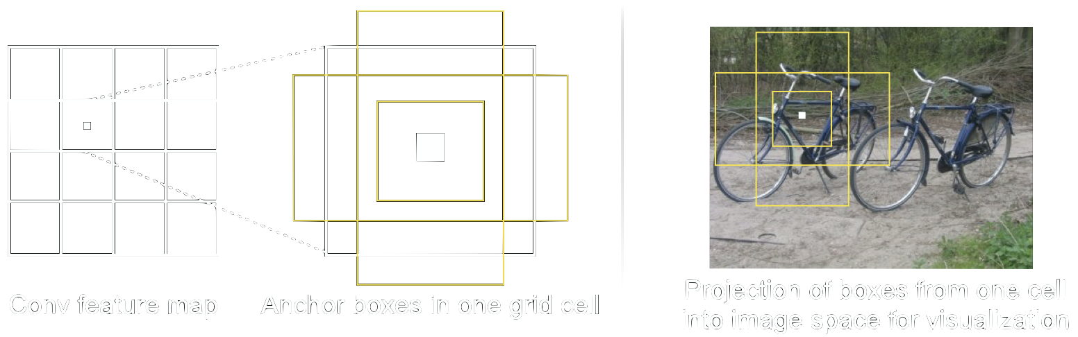
After selecting the anchor boxes we end up with a high number of overlapping, potential object locations on the feature map. For visualization we show the anchor boxes for one grid cell in the projection on the image in figure 18 on the right.
Using anchor boxes is one key ingredient in what makes Faster R-CNN faster than Fast R-CNN. Earlier versions of the R-CNN family used region proposals based on segmentation with the selective search algorithm instead [25]. While this is an intuitive way to get region proposals, it is computationally expensive. Selective search takes about \(2\)s to generate about \(2000\) proposals for an image of size \(227x227\). Using anchor boxes on the convolutional feature map allows sharing of computation between the modules 1 and 2 since the convolutional feature map is computed once only.
RPN head
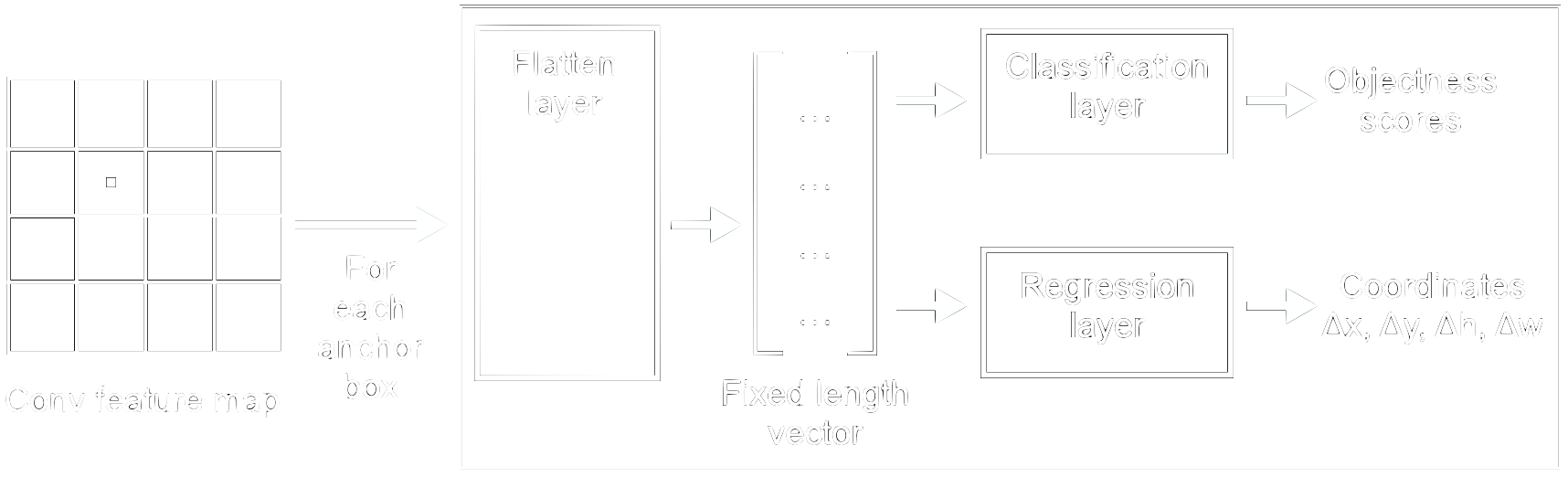
The RPN head consists of fully connected layers which take the feature map along with the anchor boxes as input and generate two sets of outputs per anchor box: objectness scores and anchor box size and coordinates relative to the grid cell centre (figure 22).
Since we are working with fully connected layers, the input has to be of fixed length. The flattening layer is therefore needed to warp the anchor box feature maps to be the same size. Here, max pooling (see the section ConvNet Basics) is applied first on the incoming anchor boxes, which are parts of varying size of the convolutional feature map, to reduce the size and get the same height and width for every input. Afterwards, this smaller map is flattened to be a one-dimensional fixed length vector. This fixed length vector is then fed in parallel into the classification and the regression layer. Here, the objectness score along with refinements to the coordinates and size of the anchor box are calculated.
The objectness score is compared with a threshold to determine if an anchor box is used as a region proposal in module 2 or not. If the objectness score is high the anchor box most likely contains an object and is kept. A low objectness score indicates that the anchor box contains no object, also called background. However, if the score is somewhere in between, the anchor box could contain a partial object. That means this anchor box is not a good reference to locate the object in module 2, and therefore it is deleted.
Post Processing - Filtering proposals
The anchor box approach still identifies far too many potential regions that could contain an object. Since the boxes overlap by design, we end up with multiple boxes identifying the same object, as illustrated on the left side in figure 23. Many of these overlapping boxes, therefore, need to be filtered out and removed.
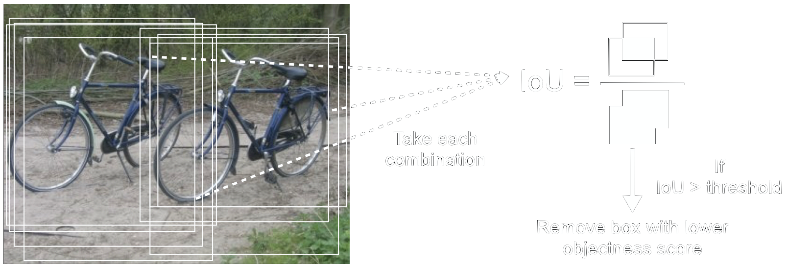
First, boxes with height or width smaller than a threshold are deleted. This discards proposals which are unlikely to contain a complete object. Next, all of the boxes are sorted by their objectness score from highest to lowest and Non-Max Suppression (NMS) is applied (figure 23). NMS first identifies boxes with high overlap by calculating their Intersection over Union (IoU). The IoU, as the name suggests, takes two boxes, calculates the area in which they overlap and divides that by the total area occupied by both boxes; thus, two anchor boxes with low IoU are more likely to represent separate objects. Conversely, two anchor boxes with high IoU have high overlap, thus are likely to represent the same object. If two boxes have high IoU, the anchor box with lower objectness score is removed. This can, however, still cause problems with objects that are partially occluded like in figure 23, so a Soft-NMS can be used instead. Here, instead of deleting the anchor box, a penalty to the objectness score is created.
The right choice of the threshold is very important for the performance of the whole detection pipeline. If the IoU threshold is too high, too many region proposals are sent to module 2, slowing the detection algorithm down. However, if the threshold is too low, good proposals are likely to be discarded, which reduces the accuracy of the final prediction.
Output - What the RPN returns
After these steps, we end up with refined, class agnostic bounding boxes for each potential object location. In Faster R-CNN, there are roughly 2000 proposals, but this number depends on the choice of parameters and can be changed according to the user’s needs.
Note here that the outputs only provide potential locations for objects. It does not provide a class label for the objects. That means if we are not interested in the specific class of the object and only a rough localization, or we have only one class, module 1 of Faster R-CNN can be used without module 2. For that the objectness scores could be further thresholded to reduce the number of proposals for example. If however, we need to distinguish between multiple object classes with low localization error we need module 2 to provide us the class labels and refine the localization.
Module 2: Detector
The second module generates the object classes and their refined positions. To accomplish this, it takes the feature map along with the region proposals from the first module. It is identical to the second module in Fast R-CNN [23]. Figure 24 illustrates the steps. All of these steps are executed sequentially for each region proposal.
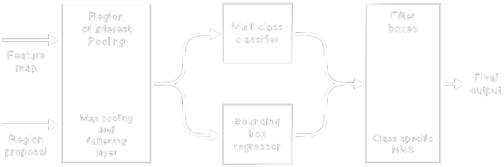
Region of Interest Pooling
The inputs to module 2 are the feature map along with region proposals of different sizes. To feed them through the fully connected layers which follow, we need to transform these inputs into vectors of fixed size. Similar to module 1, max pooling is used to warp the features from the region proposals of different sizes (hence the name region of interest pooling). Afterwards, they are flattened to get the vector of fixed length.
Notably, this warping operation is done on the feature map, not the image as in Fast R-CNN. By reusing the already computed feature map, RoI pooling saves a lot of computational effort. In the first iteration of the R-CNN architecture [26], the input image was cropped according to the region proposal first for each proposal. On each of these cropped regions, a full classifier was then applied. In addition to being computationally expensive, this method was also extremely memory intensive.
Classification and Bounding Box Regression
The fixed-size output from the RoI pooling is then fed through two fully connected layers, followed by a softmax layer. Similar to what was mentioned in section ConvNet Basics, these final layers classify the input, which in this case means for each region proposal.
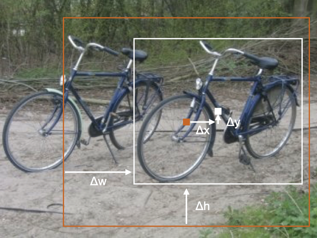
In parallel to the classifier, there is a bounding box regressor which refines the location and dimensions of each bounding box to boost the localization accuracy. This regressor outputs the adjustments on the inputted bounding box needed to better fit around the object (figure 25). This second refinement is class specific as opposed to the first one.
Class Specific Non-Max Suppression
At this point, we end up with a box with an assigned class for each region proposal. Since there are still too many possible bounding boxes, class-specific NMS is used. This time, anchor boxes with both the same class and high IoU are compared and the boxes with lower confidence scores are eliminated. This creates the final output of the network: a list of bounding boxes with their locations, dimensions, class labels, and confidence scores.
References
[22] Ren, S., He, K., Girshick, R., & Sun, J. (2016). Faster R-CNN: Towards Real-Time Object Detection with Region Proposal Networks. ArXiv:1506.01497 [Cs]. http://arxiv.org/abs/1506.01497
[23] Girshick, R. (2015). Fast R-CNN. ArXiv:1504.08083 [Cs]. http://arxiv.org/abs/1504.08083
[24] Long, J., Shelhamer, E., & Darrell, T. (2015). Fully Convolutional Networks for Semantic Segmentation. ArXiv:1411.4038 [Cs].http://arxiv.org/abs/1411.4038
[25] Uijlings, J. R. R., van de Sande, K. E. A., Gevers, T., & Smeulders, A. W. M. (2013). Selective Search for Object Recognition. International Journal of Computer Vision, 104(2), 154–171. https://doi.org/10.1007/s11263-013-0620-5
[26] Girshick, R., Donahue, J., Darrell, T., & Malik, J. (2014). Rich feature hierarchies for accurate object detection and semantic segmentation. ArXiv:1311.2524 [Cs]. http://arxiv.org/abs/1311.2524
Comments
Best explanation I’ve read so far, thank you!